LoRa mesh networks operate under one binding constraint: airtime on a shared, duty-cycled, ~kilobit-per-second channel is the only currency that matters. Meshtastic's managed flood is robust and stateless but spends the whole neighbourhood's airtime on every packet it carries; deterministic schemes promise cheaper unicast but import state that rots as nodes sleep, move and reboot. A preliminary design exploration of ours argued from first principles that a protocol should move continuously along the knowledge spectrum between flood (zero knowledge) and source routing (total assumed knowledge) and proposed gradient-corridor anycast: per-destination hop-distance gradients planted by a single flood, anycast forwarding down the gradient and an eligibility corridor that widens as the gradient ages — degrading gracefully toward flood instead of failing. Its supporting evidence was a synthetic simulation: 120 uniformly scattered nodes, invented link qualities and synthetic mobility churn.
Synthetic topologies flatter every protocol differently, so the natural objection is: does the result survive a real network? This paper answers that question using production data from RelayMesh's ingestion of the Norwegian national Meshtastic mesh, then cross-validates on five further production networks (§6.1) — to our knowledge the first evaluation of these four strategies on fully empirical LoRa mesh topologies at this scale. Along the way the real data pushes back on the design itself: an ablation (§3.6) shows the original wall-clock staleness thresholds are unnecessary and the paper's final specification is the simpler, clock-free form that survives it.
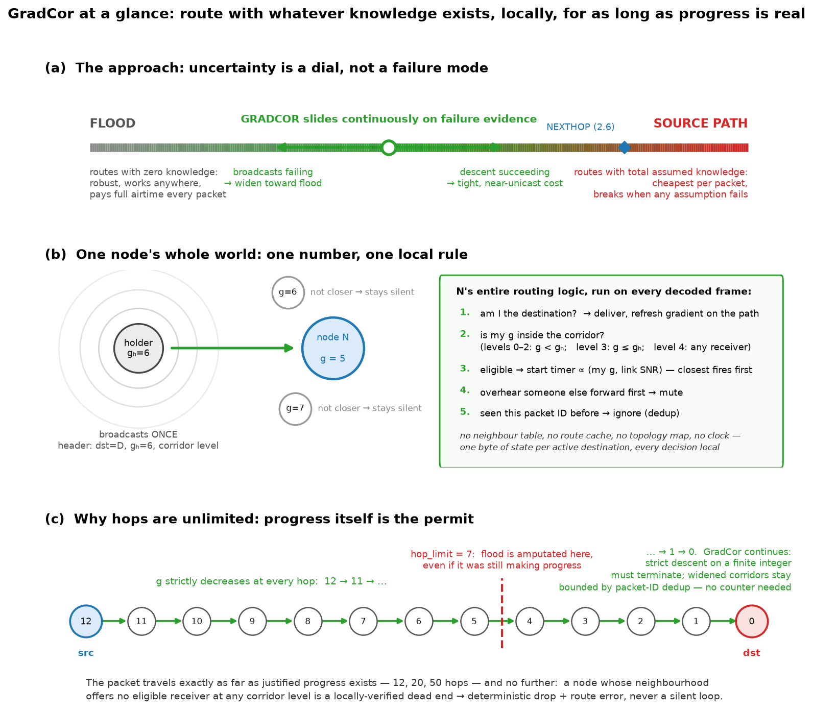
This section specifies GradCor as a protocol, independently of how we evaluate it. The design answers one question: what should a router do when its knowledge of the network is partially wrong — and it cannot know which part? Classical answers pick an endpoint: flooding assumes nothing and pays full price every time; source routing assumes everything and breaks when any assumption fails. GradCor's answer is to make the degree of trust in its own state an explicit, continuously-acting protocol parameter. Every mechanism below is an instance of that one idea and Figure 1 compresses the whole method into one picture: where the design sits (a), what any single node actually does (b) and why removing the hop limit is safe (c).
We present the method as it evolved rather than only its end state, because the simplification is itself a finding. §3.1–3.5 specify the design as originally drafted (“v1”), in which trust decays with a wall-clock age per gradient and two fixed thresholds govern corridor widening and replanting. §3.6 then ablates those clocks on the real Norwegian network and finds them redundant: the per-hop escalation already measures staleness directly. The result is the final specification, GradCor-R (“reactive”) — identical machinery with every age test deleted and one byte of state per destination — which is what we recommend implementing. Readers should take v1 as the pedagogical and historical form and GradCor-R as the protocol.
Each node keeps, per active destination only, a single pair: the estimated hop distance to that destination (the gradient, g) and, in v1, the age of that estimate. Nothing else — no next-hop pointer, no path, no per-neighbour table. This is deliberate: a next-hop pointer names one specific relay and fails when that relay sleeps; a gradient only claims “I am about N hops away,” a far weaker statement that many different neighbours can satisfy. Weak claims rot slower than strong ones. Forwarding is also independent of the node database: a relay never identifies, addresses, or decrypts for the destination — it only compares its own g against the g in the packet header — so a relay can carry traffic toward destinations it has never heard of as nodes and routing state grows with the node's active conversations, not with mesh size. Only the sending endpoint needs the destination's identity (to address the packet and encrypt), exactly as it does today.
| Field | Type | Meaning | Fate in final spec |
|---|---|---|---|
| g | uint8 | estimated hops from this node to the destination | kept — the entire routing state |
| age | uint8 (hours) | time since g was planted or last refreshed | removed by the §3.6 ablation; optional replant hint only |
On the wire, a data packet carries the destination, the normal packet ID (reused for duplicate suppression), the holder's own gradient gh and a 2-bit corridor level. That is 1–2 bytes of overhead — against a source route's full node list, this is the difference between constant and linear per-packet cost in path length.
Gradients are created by a single flood from the destination (or equivalently, by the reverse view of any flood the destination originates — in Meshtastic practice, a NodeInfo, position, or ordinary channel-message broadcast can double as a planting flood at zero extra cost). There is no dedicated announce packet type and no transmission the mesh would not otherwise carry: planting is a side effect of whatever the destination already sends. Every node the flood reaches records the hop count at which it first heard it: that is the gradient, age zero. One broadcast per node, once, amortised over every subsequent packet toward that destination. There is no periodic beaconing; the protocol never spends airtime maintaining state it is not using. This side-channel turns out to be the load-bearing one. Production broadcast cadence puts a typical Norwegian node's own broadcasts about an hour apart (§6.13), so gradients toward it are re-planted hourly by traffic the mesh sends regardless — and §6.13 shows the protocol's advantage tracks that cadence closely. GradCor adds no announce mechanism, but it is not independent of the mesh having one: it inherits Meshtastic's. Nor does a gradient-less source need to solicit a plant: it can managed-flood the packet exactly as Meshtastic does today and if that flood delivers, the refresh of §3.5 plants the gradient along the proven path for every packet after it — the replay's on-demand planting shortcut and this deployable cold start are compared quantitatively in §8. Figure 2 traces the two numbers through their whole life: stamped by the planting wave (a), sitting as a two-byte table row (b) and re-stamped for free whenever a delivery proves what the true working distance is (c).
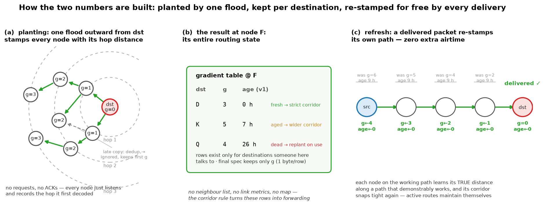
One honest subtlety: the planting flood travels outward from the destination, while data flows toward it — and §4 shows 43% of real links have no observed reverse. The gradient is therefore a distance estimate measured partly over links the data cannot use in reverse: g can underestimate the true forward distance and a strictly-descending chain from g=4 can never be longer than five nodes. GradCor survives this for two reasons. First, forwarding is anycast — it never needs the specific reverse of any planting hop, only some decoded receiver with a lower g. Second, the corridor widens per hop, not only with age: a holder that finds no strictly-closer receiver retries, then admits equal-g receivers, then any receiver (Algorithm 1), so an optimistic gradient degrades into guided exploration rather than failure — and the moment one packet gets through, the delivery refresh (§3.5) re-stamps every node on the working path with its true forward-path distance, converting the exploration cost into a one-time fee per gradient lifetime. In the Norway replay this is measurable: 22.8% of gradient-guided deliveries took more hops than the sender's g promised (median one extra, maximum +19) and when g strictly underestimated the true reachable distance, packets still got through at a degraded rate (16% vs 64% baseline) at roughly 6× the airtime — degraded, not dead and self-correcting on first success. The evaluation in §5–6 replays this asymmetry faithfully rather than assuming it away.
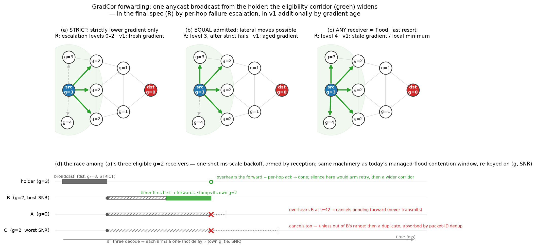
The holder of a packet does not pick a next hop. It broadcasts once and eligibility is decided at the receivers: every node that decodes the frame compares its own gradient with the gh in the header. Eligible receivers start a contention timer proportional to their gradient (ties broken by link quality); the timer that fires first forwards the packet and the other candidates hear that forward and suppress themselves. One clarification to carry through the rest of the paper: this contention timer is a one-shot, milliseconds-scale MAC backoff armed by a packet reception — a race resolver, not a clock. It is unrelated to the hours-scale state-aging clocks that §3.6 later removes and it is intrinsic to anycast: some tie-breaker must decide which eligible receiver goes first. This is the ExOR trick[2], and it is what converts LoRa's broadcast medium from a liability into the protocol's main asset: one transmission simultaneously probes every potential relay, so the packet advances if any of them is awake and heard it — where unicast schemes stall if the named one didn't.
Two mechanics deserve spelling out, because both differ from the hop-count intuition a reader may carry in. First, gh is not a TTL: no one decrements it. Each forwarder overwrites the field with its own stored gradient before rebroadcasting, so the header always reads “the current holder believes it is N hops away.” Under the strict rule the value falls at every hop — which is what provides the termination a TTL normally buys — but it falls because each node stamps its own better knowledge, can snap downward mid-flight when the packet reaches a node with a shortcut and (in the widened corridors) may hold or rise where a countdown would already have killed the packet. Second, the winner's forward transmission is itself the per-hop acknowledgment: the holder overhears it and goes quiet — the same passive-ack-by-rebroadcast the managed flood uses today, so no explicit ACK packet exists at any hop. Silence within the contention window is therefore the holder's failure signal and it is exactly what arms the escalation of §3.4: hear nothing, retry; still nothing, widen the corridor and broadcast again. Figure 3(d) traces one complete race on the time axis.
send(src, dst):
  if no gradient for dst at src or age ≥ AGE_DEAD (24 h):
      plant(dst)                          # one flood from dst; abort if src unreached
  holder ← src;  visited ← {src}

  loop:
      for level in 0..4:                  # at most 5 broadcasts per hop
          corridor ← STRICT  if level ≤ 2 and age < AGE_WIDEN (3 h)
                     EQUAL   if age ≥ AGE_WIDEN or level = 3
                     ANY     if level = 4
          broadcast(pkt, g_holder, corridor)                # one airtime unit
          # at each receiver v ∉ visited that decoded the frame:
          if v = dst:                     deliver; refresh gradient along path; return
          eligible(v) ↔  g(v) < g_holder            (STRICT)
                       |  g(v) ≤ g_holder            (EQUAL)
                       |  v decoded the frame         (ANY)
          if any eligible: winner ← contention race (min g, then best SNR); break
              # losers mute on overhearing the winner — its forward
              # is the holder's implicit ack (Figure 3d)
      if no winner: drop deterministically  # local minimum; RERR toward src (§3.5)
      visited ← visited ∪ {winner};  holder ← winner
visited set is not carried in the packet: Meshtastic's existing packet-ID duplicate
suppression plays the same role, since a node that already forwarded a packet ignores it
thereafter. Note the key is forwarded, not seen: a contention loser that muted
(Figure 3d) never transmitted and must stay eligible for later broadcasts of the same
packet — §3.7 explains why this distinction carries real recovery value.The corridor rule is the novel piece and the reason the protocol has no cliff-edge failure mode (Figure 3). While the gradient is fresh (<3 h), only strictly-lower-gradient receivers may forward: the packet monotonically descends toward the destination at near-unicast cost and the strict decrease on a finite integer proves both loop freedom and termination without any hop-limit counter. As the gradient ages past 3 h — knowledge now suspect — equal-gradient receivers are admitted, buying lateral moves around a sleeping relay or a newly-dead link at modest extra cost. If even that fails, or the gradient is very old, any receiver qualifies: the packet is now effectively flooding, which is exactly the right behaviour when the node knows nothing — and it is reached gradually, hop by hop, not by a mode switch that must itself be signalled. The widening is strictly local: the source never decides to “send as flood,” and a corridor opened to ANY at one troubled hop does not stay open — the next holder starts again at STRICT, so the packet re-tightens the moment it is past the gap. Uncertainty in GradCor is not an error state; it is a dial that trades airtime for reach in proportion to how much the state deserves to be trusted. Note that v1 drives this dial with two triggers — wall-clock age and per-hop failure escalation — which are redundant with each other; §3.6 shows the per-hop trigger alone carries the whole effect on the real network and the final specification keeps only it.
Delivery is itself the maintenance protocol. When a packet reaches the destination, every node on the path it took is stamped with its true distance-to-destination along that working path, age zero (Figure 2c; in firmware this rides the existing delivery ACK). Active conversations therefore keep their own gradients fresh for free and the corridor stays tight exactly where traffic flows — the state/freshness trade-off (§1) is paid only for destinations nobody is talking to. This mechanism is real but, on production traffic, it is the minor one. §6.13 measures the actual addressed-traffic process and finds most pairs exchange a single isolated packet, so there is usually no second packet for a delivery refresh to help; what actually keeps gradients fresh is the other free-planting source, §3.2's — the destination's own routine broadcasts, which production data shows arrive roughly hourly. The design does not change, but the reason it works does, and it is worth stating plainly here rather than leaving the reader with the wrong model. One asymmetry consequence is worth naming: the confirmation travels its own reverse path, which on an asymmetric mesh need not retrace the data's forward path — forward-path nodes out of earshot of the return leg simply miss that refresh. The miss is benign by construction: a node that misses a refresh merely keeps a staler g — there is no named next hop to be wrong about — and the cost is a little extra escalation on a later packet, precisely the failure the §3.3/§3.4 ladder absorbs (the replay's idealization of this refresh is disclosed in §8, item 6). A gradient that reaches 24 h without a refresh is declared dead and the next send replants it; Figure 4 summarises the states.
In the final specification the lifecycle therefore simplifies as the lower band of Figure 4 shows: the delivery refresh survives unchanged, the FRESH/AGED/DEAD clock states disappear because eligibility no longer consults age and replanting degenerates to “plant if you have no gradient at all” (an optional coarse timer may evict rows that have not been refreshed for days, purely as memory hygiene).
The drop rule completes the lifecycle. A packet whose holder finds no eligible receiver at any corridor level is at a locally-verified dead end: across the whole escalation ladder — strict, equal, any — no un-visited receiver decoded the packet at all. It drops the packet there, deterministically and can report a route error back toward the source (the RERR is specified but not exercised in §6's evaluation). Contrast both alternatives: a hop-limit expiry drops at an arbitrary distance-driven point regardless of progress and a stale unicast route black-holes silently. GradCor's failure is localised, observable and actionable — the property the original design brief demanded when it argued for removing the hop-limit counter, with the packet's lifetime bounded instead by the visited-set/dedup rule and the finite gradient descent.
Two constants in the specification look like magic numbers: widen at 3 hours, replant at 24.
A fair objection is that these are statically chosen and the soft-state literature suggests
the “right” staleness timer should track the measured hazard rate of state
invalidation — the reasoning behind RPL's Trickle timer[6], which resets on
observed inconsistency rather than on a schedule. We therefore ablated the clocks on the
Norway replay (experiment_widening.py; Figure 5).
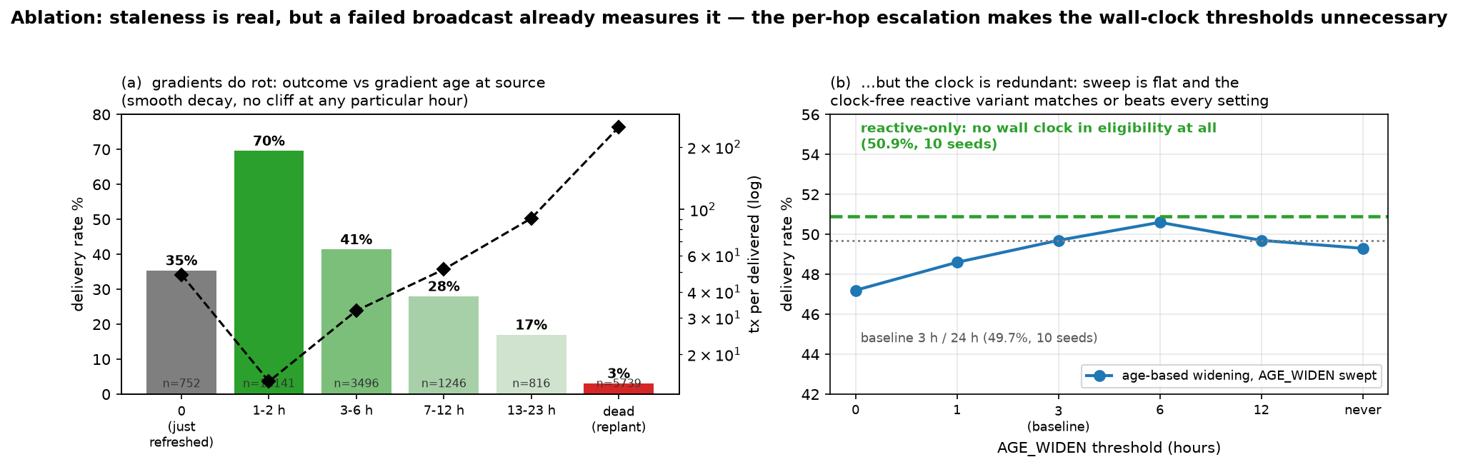
Three findings. First, staleness is real: delivery through a 1–2-hour-old gradient runs at 70%, decaying smoothly to 17% at 13–23 hours with airtime cost rising in step (Figure 5a) — a genuine hazard process with no cliff at any particular hour, so no specific threshold is “correct.” Second, the wall-clock threshold barely matters: sweeping the widening age from 0 (always widened) to never-widen moves delivery only between 47.2% and 50.6% (Figure 5b). Third, the clock is redundant: a variant that removes wall-clock age from the eligibility rule entirely — per-hop escalation only, strict → equal → any — delivers 50.9% vs the 49.7% baseline over 10 seeds, at equal cost; even deleting the replant timer too leaves it at 50.9%. The explanation is that a failed anycast broadcast is a direct, local measurement of the exact staleness the clock tries to predict: the age threshold decides in advance what the next three transmissions will discover anyway. Following the same Trickle logic, reacting to the inconsistency beats scheduling it — and the “two numbers” of §3.1 reduce to one (age survives only as an optional, insensitive replant hint). We also tested one adaptive variant in the opposite direction — a learned per-destination starting level that skips strict attempts a previous packet did not need — and it is worse (43.1%): skipping the cheap strict probes forfeits their frequent wins. The simple deterministic rule survives its own ablation; the statistical refinement does not.
This yields the final specification — what the design evolved to. It is Algorithm 1 with every age test deleted, nothing more:
# GradCor-R (final specification): Algorithm 1 with the clocks removed.
# State per active destination: g only (one byte + key). No aging tick.
send(src, dst):
  if src has no gradient for dst:
      plant(dst)                          # one flood; the only replant rule
  loop over holders as in Algorithm 1:
      for level in 0..4:
          corridor ← STRICT (g < g_holder)  if level ≤ 2
                     EQUAL  (g ≤ g_holder)  if level = 3
                     ANY                     if level = 4
          broadcast; receivers race exactly as before;
          delivery refreshes g along the path
      if no winner: drop deterministically + RERR      # unchanged
Each ingredient is individually proven: monotone-metric descent is Babel's feasibility condition[3] and RPL's rank rule[4]; receiver-side anycast with contention timers is ExOR[2]; destination-rooted gradients go back to directed diffusion in sensor networks. The composition is what is new: coupling eligibility width to the protocol's own evidence of staleness — wall-clock age in v1, per-hop failure escalation in the final spec — so the protocol occupies the whole flood↔unicast spectrum continuously instead of switching between brittle modes and refreshing its state opportunistically from delivered traffic instead of periodic control packets.
A Meshtastic port is less invasive than it may sound. The firmware's router hierarchy
(src/mesh/FloodingRouter → NextHopRouter) already contains the
two hard primitives: packet-ID duplicate suppression (the visited set) and an SNR-weighted
rebroadcast contention window (RadioInterface::getTxDelayMsecWeighted) — the
managed flood already makes far nodes rebroadcast first; GradCor re-keys that same timer on
(gradient, SNR). The gradient table is a small addition to per-node state alongside the
NodeDB, planting piggybacks on floods that already happen (NodeInfo, position) and the
corridor level fits in spare header bits. Porting GradCor-R rather than v1 removes every
scheduled timing element: no per-entry aging tick, no periodic timer, no state clock. The
one timer that remains is the contention backoff of §3.3 — one-shot, milliseconds
scale, armed only by a reception — and the firmware already ships its exact skeleton:
getTxDelayMsecWeighted maps the received SNR to a contention-window size
(−20…10 dB → CWmin…CWmax), gives
ROUTER-role nodes an early window and picks a random slot inside it. GradCor-R re-keys the
slot choice on (gradient, SNR) instead of SNR alone; no new timing machinery is introduced.
The genuinely open engineering risk is contention-race correctness when several eligible
receivers sit inside mutual capture range — duplicate forwards cost airtime but are
absorbed by dedup; missed suppression is the case to instrument first (§8, item 5).
One dedup semantic needs deliberate care in the port. Meshtastic's
wasSeenRecently drops a packet the node has seen; GradCor's visited-set
equivalent must drop only what the node has forwarded. The difference is the protocol's
self-recovery path: a contention loser that muted (§3.3) has seen the packet but never
carried it — if the winner's branch dead-ends a few hops later and a widened-corridor
broadcast reaches that loser again, it must be allowed to pick the packet up. Under seen-keyed
dedup every raced-and-lost candidate is permanently consumed and a packet that commits to a
failing branch cannot wander back to the branch that would have worked; under forwarded-keyed
dedup only the actual chain of forwarders is burned. The replay models forwarded-keyed dedup
throughout and its recovery behaviour is visible in the data — 22.8% of gradient-guided
deliveries took more hops than the sender's gradient promised (§3.2), i.e. walks that
detoured and still arrived. A seen-keyed port would silently forfeit exactly those deliveries;
the change is one predicate, but it belongs on the firmware-prototype checklist next to the
contention race.
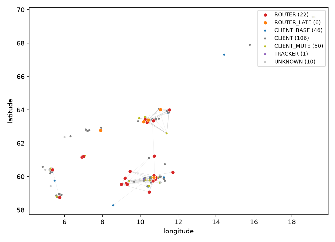
All inputs were extracted from RelayMesh production systems for network “norway” (a public community network) over 2026-06-27 → 07-04:
| Source | Content | Volume |
|---|---|---|
| Memgraph (topology graph) | :Node rows of the 7-day build window (roles, GPS; its pre-fix :HEARD edges were not used — see below) | 499 nodes, 3,613 edges |
ClickHouse messages | raw TRACEROUTE_APP packets (fwd path, route_back, per-link SNR) | 18,919 packets |
ClickHouse node_activity_5min | per-node hourly message counts (presence) | 326 active nodes |
Extracting links from traceroutes requires one correctness step the production topology builder
missed at the time of this study: 31% of stored TRACEROUTE_APP rows are responses, not
requests. A response is a new packet whose envelope source and destination are swapped while
route[] still lists the relayers in requester→responder order; parsing it as a
request creates reversed edges and parsing mid-flight rows as complete paths invents endpoint
hops that never happened. The corrected extraction — developed alongside this paper and
since shipped to RelayMesh production — classifies each row by payload shape
and hop accounting, orients both legs correctly and appends endpoints only on arrival
evidence. The effect is large: the naive parse yields 4,249 directed links, the
corrected one 1,423 — and measured link reciprocity rises from 36% to 57%,
i.e. much of the apparent asymmetry in the production graph is an extraction artifact, though
43% of real links still have no observed reverse. Return legs (route_back),
previously discarded in production, contribute 303 links (~21%) seen in no other way. Role distribution:
141 CLIENT, 66 CLIENT_MUTE, 55 CLIENT_BASE, 24 ROUTER, 6 ROUTER_LATE, 1 TRACKER, 206 unset. The
largest weakly connected component covers 200 nodes, the largest strongly connected component
125 and the graph is hub-dominated: the busiest routers (degree 53–107) anchor the
geographic clusters.
The study is a trace-driven replay: rather than inventing a radio environment, we reconstruct the network the production pipeline actually observed — which links existed, how good they were and when each node was awake — and then run all five forwarding protocols (the four strategies of §2, with GradCor in both its v1 and final form) over that reconstruction, hour by hour, for the same week the data describes. Figure 7 shows the pipeline end to end; the subsections below walk through each stage.
Meshtastic's traceroute is the only mechanism in the production data that reveals individual
RF hops. A traceroute request floods toward its destination; every node that relays it
appends itself to the packet's route[] array and records the SNR at which it heard
the previous hop in snr_towards[]. The responder then emits a new packet
— envelope source and destination swapped, route[] copied unchanged, its own
return relayers accumulating in route_back[]/snr_back[]. The true
forward path of the probe is therefore [requester] + route + [responder] and every
consecutive pair in that sequence is one real, directed, SNR-annotated radio reception
(Figure 8). Three correctness rules matter (each was validated against the raw data):
responses are detected by payload shape and hop accounting and their legs oriented
requester→responder regardless of envelope direction; endpoints are appended only when the
SNR array proves the leg actually arrived (mid-flight copies heard by a gateway must not invent
the final hop); and duplicates, broadcast and placeholder IDs are dropped. The response
heuristic is needed because the canonical discriminator — the protobuf
request_id — is absent from encrypted rows (~98% of traffic); on the recent
unencrypted rows where it is present, the heuristic matches the canonical label on
98.7% of 871 ground-truth responses. Because part of that heuristic is hop accounting, it
depends on hop_start being present and truthful; the 2.8 line proposes dropping
packets with a missing or invalid hop_start[8], which would make this anchor
strictly more reliable on future windows than on ours.
[requester]+route+[responder], whose consecutive pairs are
real SNR-annotated receptions. Dashed red: the return leg from route_back, which
travels different links when the mesh is asymmetric. Parsing both legs of all 18,919 rows with
correct response orientation yields 1,423 distinct directed links; the return legs alone
contribute 303 (~21%) that the pre-fix production builder discarded.Aggregating across all packets, each directed link (u→v) accumulates an observation count and a mean SNR. Direction is radio direction: u transmitted, v decoded. This graph is deliberately not symmetrized — asymmetry is a finding, not noise (§4).
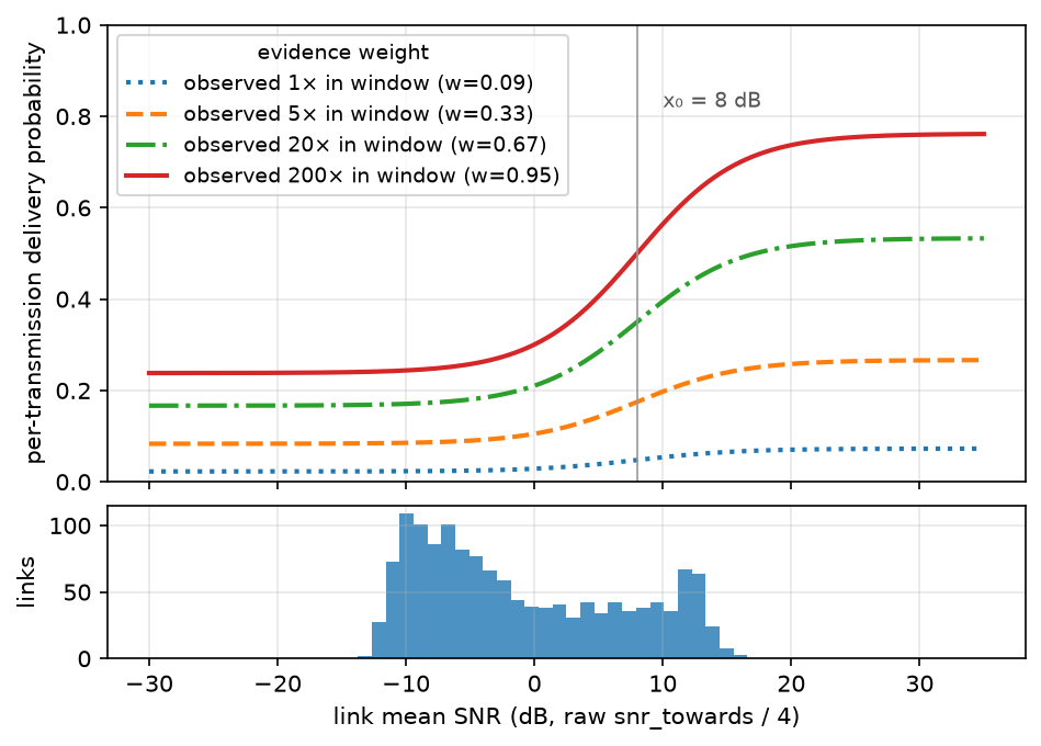
The trace tells us a link existed; a simulation additionally needs the probability that a single transmission on it succeeds. We model this with two multiplicative factors (Figure 9):
p(u→v) = w · [ pmin + (pmax − pmin) / (1 + e−(SNR − x₀)/4) ],
w = obs / (obs + k)
The bracket is a logistic packet-success curve in the link's mean measured SNR (raw
snr_towards divided by 4 to approximate dB): strong links approach
pmax, weak ones fall toward pmin. The evidence weight w
encodes a different fact: a link observed once in seven days — a ducting event, a moment
of antenna alignment — is not a dependable link, however good its single SNR sample
looked, while one observed hundreds of times is infrastructure. Without this term the simulator
treats every fleeting link as permanently available and over-delivers dramatically at short hop
counts.
Because reverse directions could be under-observed, the model includes an optional prior: an
unobserved reverse link (v→u) may be granted rev_p · p(u→v)
rather than zero, with rev_p calibrated rather than assumed. As §5.3 shows, the calibration
drove rev_p to zero — once response rows are oriented correctly, the observed round-trip
rate is already explained without inventing reverse links.
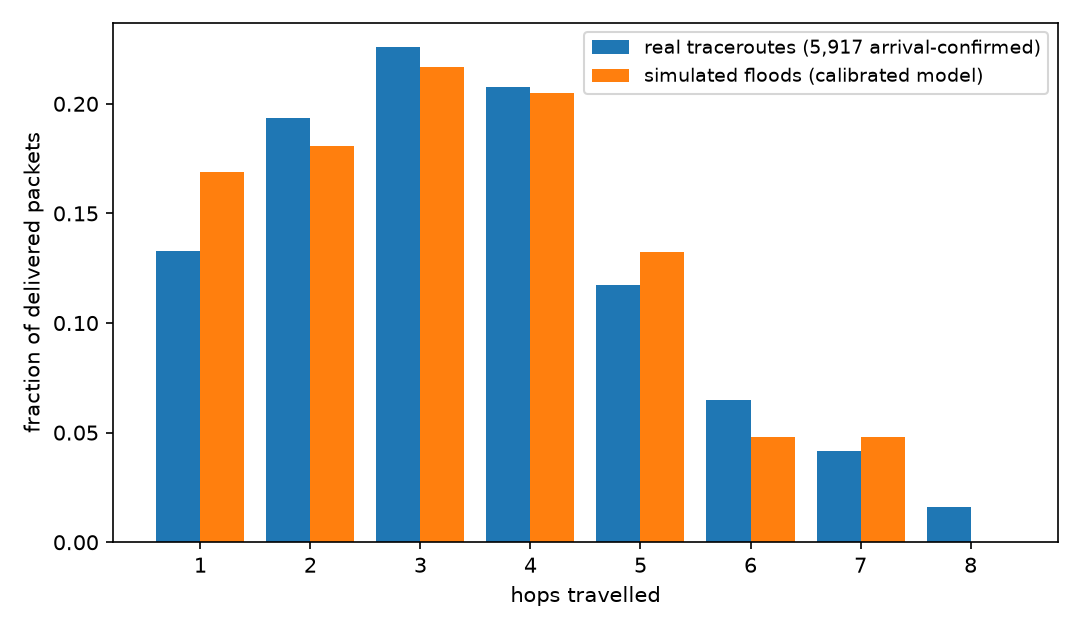
The model has five free parameters (x₀, pmax, pmin, k, rev_p). None are hand-picked: all were grid-searched to jointly minimise the distance to two statistics the trace itself provides.
route_back,
i.e. completed the round trip. Simulated forward-then-reverse floods between the same pairs must
approximate this rate. This anchors reverse-link generosity — exactly the quantity PATH's
viability depends on.
Best fit: x₀ = 8 dB, pmax = 0.8,
pmin = 0.25, k = 10, rev_p = 0. Both anchors now fit
well (Figure 10; round trip 0.31 simulated vs 0.23 real). One denominator caveat: the two
round-trip rates are not the same statistic — the real 23% is the share of all observed
traceroute rows carrying a route_back, while the simulated 31% is the fraction of
delivered forward floods whose reverse flood also delivered — so this anchor is
directional rather than exact. Under either reading the simulator treats reverse paths at least
as generously as the trace shows, the direction that can only flatter PATH (§8, item 1).
Notably the grid chose
rev_p = 0 — with correctly-oriented links, the data is best explained by
unobserved reverse directions simply not existing, so asymmetry is fully binding in the
replay. The small remaining round-trip optimism can only overstate PATH (§8).
The synthetic study modelled churn as random node movement. The production data says the real phenomenon is duty cycling: the median Norwegian node was online 22 of 168 hours and the 90th percentile 167. We therefore give every node a set of online hours — the union of its hourly activity buckets and its appearances inside any traceroute path, with gaps of ≤3 hours filled (a node relaying at 09:00 and 11:00 was almost certainly on at 10:00). A node that is offline in a given hour cannot receive, relay, or originate. This is a stronger and more honest stressor than mobility: state rots not because topology changed shape but because the node holding the route simply went to sleep.
All five protocols run over the identical world model; none is given information the others lack. Table 2 lists the fixed parameters. FLOOD and the discovery/fallback floods inside the other four protocols share one implementation, including a first-order MAC model: when several copies of a packet arrive at one receiver in the same flood round they collide and the strongest frame survives with capture probability 0.8 (otherwise all are lost). CLIENT_MUTE nodes never rebroadcast in any protocol.
| Parameter | Value | Applies to |
|---|---|---|
| Hop limit | 7 | all floods |
| Per-hop unicast retries | 3 | PATH, NEXTHOP |
| Extra strict-corridor broadcast tries | 2 | GRADCOR v1 & R |
| Corridor widens at gradient age | 3 h | GRADCOR v1 only |
| Gradient replanted at age | 24 h | GRADCOR v1 only |
| Collision capture probability | 0.8 | all floods |
| Safety cap, transmissions per packet | 2,000 | all protocols |
sim_norway.py).
The hop limit is set to Meshtastic's protocol ceiling of 7 rather than the shipped default of 3
— a choice that favours FLOOD, PATH and NEXTHOP, whose reach it bounds. Planting floods
obey the same limit, so the replay never exercises gradient descent beyond 7 hops: the
unlimited-hop property of §3 is a spec-level guarantee, not something this evaluation
stresses. The limit's value matters asymmetrically for GradCor's internal floods
(experiment_hoplimit_flood.py): raising it to unlimited gains almost nothing
(50.9 → 51.3% and an unlimited flood costs only ~9% more transmissions than
hop-7, since dedup already bounds it), but lowering it to the shipped default of 3 starves
planting reach and costs 13 delivery points (50.9 → 37.9%).PATH discovers a route with one flood, returns the recorded path hop-by-hop over the reverse links (the discovery fails if the reply dies), then source-routes data strictly along the path with 3 tries per hop; a broken hop invalidates the route and permits one rediscovery per packet. NEXTHOP keeps, at every node, the relay that last delivered a packet toward each destination — learned free of charge from the parent chain of any successful flood — and chains down these caches, falling back to a flood (which re-teaches caches) on any miss or per-hop failure. GRADCOR v1 implements Algorithm 1 exactly as specified in §3, with gradient ages advancing once per simulated hour (the upper band of Figure 4); GRADCOR-R implements Algorithm 2, the clock-free final specification. Both run in parallel in the head-to-head so the evolution claim of §3.6 is tested in the same arena as the competing protocols, not only in isolation. For both, the contention race is resolved ideally (lowest gradient always wins, suppression never fails) — a simplification whose consequences are discussed in §8. A second GradCor-specific shortcut also needs flagging: a source with no gradient triggers the planting flood from the destination at that instant, charged to the triggering packet. Causally, nothing in a deployment tells a destination to flood on demand; the deployable cold-start paths are seeding by the destination's ordinary periodic broadcasts and the flood-the-packet fallback of §3.2. §8, item 7 replaces the shortcut with both deployable forms and measures the difference.
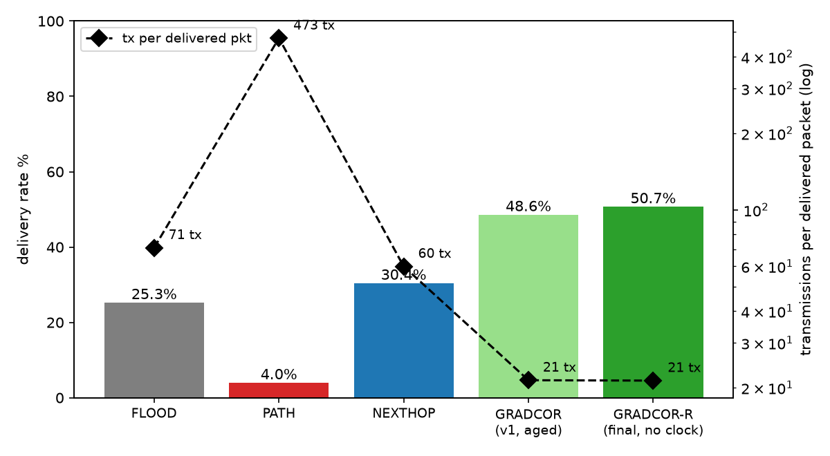
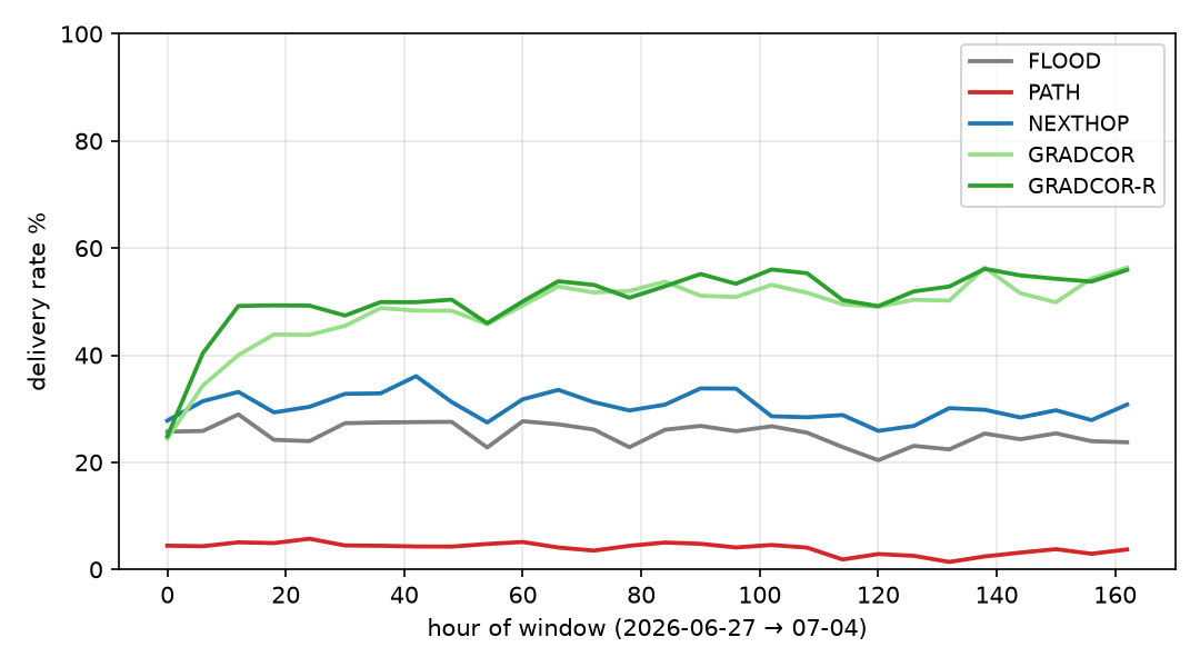
Traffic draws its pairs from the real demand pattern: 30 (source, destination) pairs sampled from the actual traceroute pair-frequency distribution (weighted, without replacement), restricted to endpoints online ≥20 hours in the week so conversations can exist at all. Its cadence, however, is a modelling choice and not a measurement: each pair sends one packet per hour, but only in hours where both endpoints were genuinely online — a message to a sleeping node is not a routing failure and must not be scored as one. That metronome is roughly 90× denser than production addressed traffic, and §6.13 measures the real process and re-runs the headline under it. The results in §6 through §6.12 should be read as holding at this fixed, generous conversational density; §6.13 states what changes when it is replaced with the measured one, and it changes the explanation of the result more than the result. Ten seeds give ≈30,000 packet attempts per protocol. Every broadcast or unicast attempt costs one transmission; gradient-planting, discovery and fallback floods are charged to the packet that triggered them, so no protocol externalises its control traffic. We report delivery rate, transmissions per packet sent (offered-load cost) and transmissions per packet delivered (the airtime price of a success — the currency that matters, per §1).
| Protocol | Delivery % | Tx / packet sent | Tx / packet delivered |
|---|---|---|---|
| FLOOD (hop limit 7) | 25.3 | 17.9 | 71.0 |
| PATH (stylized source routing, §2) | 4.0 | 18.9 | 473.2 |
| NEXTHOP (2.6-style cache) | 30.4 | 18.2 | 59.9 |
| GRADCOR v1 (age-widened corridor) | 48.6 | 10.4 | 21.4 |
| GRADCOR-R (final spec, no clocks) | 50.7 | 10.8 | 21.3 |
A single network, however real, is one draw from the space of mesh topologies. To test whether the result is a property of the protocol or a property of Norway, we ran the identical harness on the five other production networks with the most traceroute traffic in the same week: Bay Area Mesh (3,637 nodes), Florida Mesh, SoCal Mesh, Meshtastic Portugal and Meshtastic Italia. Everything was recomputed from scratch per network — link graph, presence, roles and crucially the link-model calibration, re-fitted against each network's own hop-count distribution and round-trip completion rate (the fitted parameters genuinely differ: x₀ ranges 0–12 dB and the reverse-link prior stays at zero everywhere except Florida and SoCal). Reusing Norway's constants elsewhere would have been methodologically wrong; nothing about the protocols themselves was changed or tuned.
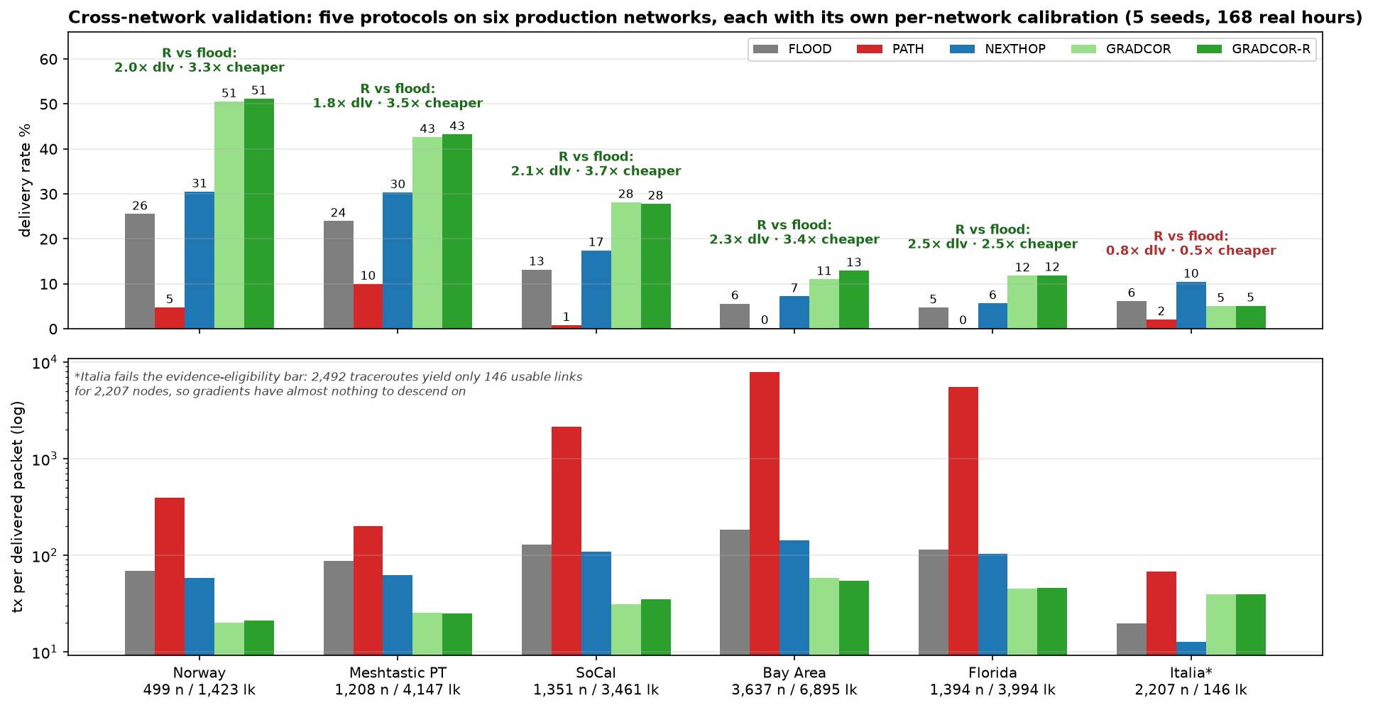
| Network | Nodes | Links | Recip % | FLOOD % | GRADCOR-R % | R vs flood | R tx/dlv |
|---|---|---|---|---|---|---|---|
| Norway | 499 | 1,423 | 57 | 25.5 | 51.2 | 2.0× @ 3.3× cheaper | 21.3 |
| Meshtastic PT | 1,208 | 4,147 | 36 | 24.0 | 43.2 | 1.8× @ 3.5× cheaper | 25.1 |
| SoCal Mesh | 1,351 | 3,461 | 31 | 13.2 | 27.8 | 2.1× @ 3.7× cheaper | 35.2 |
| Bay Area Mesh | 3,637 | 6,895 | 32 | 5.6 | 12.9 | 2.3× @ 3.4× cheaper | 54.3 |
| Florida Mesh | 1,394 | 3,994 | 37 | 4.7 | 11.9 | 2.5× @ 2.5× cheaper | 46.1 |
| Meshtastic Italia | 2,207 | 146 | 30 | 6.2 | 5.1 | 0.8× — below eligibility bar | 39.9 |
multinet_results.csv). Norway's row is its 5-seed re-run within
this harness, hence the small differences from Table 3's 10-seed values — a useful
incidental read on seed noise (≈±0.5 points). Absolute delivery scales with
evidence density — the dense US networks have far more nodes per usable link, so every
protocol delivers less there — but the ratios hold. Italia's row is the operative
precondition, not a counterexample: gradient routing needs enough traceroute-derived link
evidence to plant gradients on — exactly the evidence the extraction fixes of §7
(now shipped) increase.Two observations deserve emphasis. First, the ranking and the ratios — the two things §8 argues are the trustworthy outputs of this methodology — survive a 7× range in network size, a 30–57% range in link reciprocity and independently fitted link models; the Norway result is not a topology accident. Second, the one failure is diagnostic rather than embarrassing: where traceroute evidence is too thin to define gradients (Italia, 0.07 links per node), GradCor degrades to roughly flood performance instead of below it — the graceful-degradation property doing exactly what it was designed to do at the extreme — while the evidence-free NEXTHOP cache takes the lead. Evidence density is thus a measurable eligibility criterion for deploying gradient routing on a given mesh.
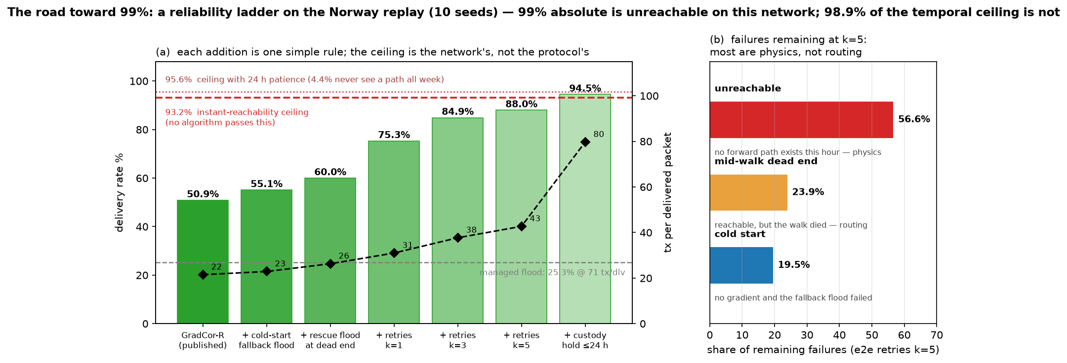
A natural next question is how far delivery could be pushed — say, to 99%. The replay can
answer this honestly because it can first measure what no algorithm can exceed: the fraction of
attempts for which a forward path over online, relay-capable nodes exists at all. On the
Norway world that instant-reachability ceiling is 93.2% and patience barely moves it: a
packet held and retried for up to 24 hours can reach at most 95.6% of attempts, because
4.4% of them never see a forward path in the entire week
(experiment_target99.py, experiment_custody.py; 10 seeds). 99%
absolute delivery is therefore not a protocol problem on this network — it is
unreachable by any routing scheme whatsoever — and the meaningful question becomes
distance to the ceiling.
That distance can be closed almost entirely with three additions, each a single rule that leaves the one-byte state and the forwarding walk untouched (Figure 14a). First, the fallback-flood cold start already measured in §8, item 7 (+4 points). Second, a rescue flood at the local minimum: instead of the deterministic drop, the stuck holder floods the packet from where it stands (+5 points) — philosophically consistent, since the drop point is by construction the node that has just proven, across the whole escalation ladder, that its knowledge is exhausted and a flood from there is the narrowest flood that can still help. Third — the single biggest lever — end-to-end retries: re-sending the packet up to k times on failure lifts delivery to 75.3% (k=1), 84.9% (k=3) and 88.0% (k=5), i.e. 94.4% of everything reachable. Each retry draws fresh channel outcomes and benefits from whatever gradients the failed attempts refreshed; the machinery is not hypothetical — Meshtastic's reliable-delivery layer already retransmits unacknowledged DMs today and the headline evaluation deliberately granted no protocol this help (§8, item 8). Finally, custody — holding a failed packet and retrying hourly for up to 24 h, the one genuinely new architectural element (a store-and-forward queue with expiry) — reaches 94.5%: 98.9% of the temporal ceiling. The anatomy of what still fails at k=5 confirms the diagnosis (Figure 14b): 56.6% of remaining failures are physically unreachable that hour, versus 23.9% mid-walk losses and 19.5% failed cold starts.
The price is stated just as plainly: transmissions per delivered packet rise from 21.5 (published spec) to 42.7 at k=5 and 79.7 with custody — at the extreme, airtime per delivered packet returns to flood's level (71) while delivering 3.7× more. The efficient knee is k=3–5 without custody: 85–88% delivery at 38–43 tx per delivered packet, still well ahead of flood on both axes simultaneously. Three caveats bound the claim: the replay's independent per-transmission link draws flatter retries relative to real correlated fading (§8, item 8); no duty-cycle budget is modelled and 38–75 transmissions of offered load per packet may be regionally infeasible; and custody changes the application contract (deliveries arriving hours late). The structural conclusion survives all three: simple reliability envelopes take GradCor essentially to the network's own ceiling, and the ceiling itself — the last five to seven points — is an operations problem, router coverage and evidence density, the same deployment precondition §6.1's evidence-starved network surfaced.
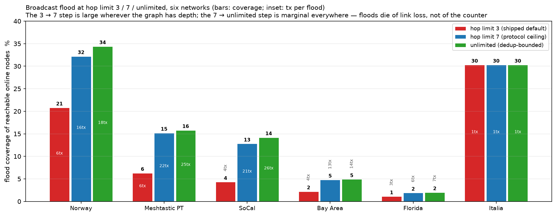
GradCor removes the hop limit only where strict descent certifies progress — unicast. The
majority of a mesh's load (positions, telemetry, NodeInfo, channel texts) is broadcast and
keeps managed flooding (§8, item 9), so a fair question is whether that traffic
could shed its hop limit too. Structurally it can, safely: duplicate suppression, not the
counter, is what terminates a flood — every node relays a given packet at most once, so
an unlimited flood is bounded by mesh size. Whether it is worth anything is an
empirical question and the answer across all six networks is: almost nothing
(experiment_hoplimit_multinet.py, Table 5). Raising the limit from 7 to
unlimited adds at most 2.2 points of reachable-node coverage (Norway) for 11–25% more
transmissions; on four of the six networks the gain is under one point. The limit does still
bind at 7 — on 8–38% of floods the frontier is alive when the counter cuts
it — but that surviving frontier is so attenuated by per-link loss that letting it run
adds little. Floods die of link loss, not of the counter.
The consequential knob sits at the other end: Meshtastic's shipped default of 3. On every network with usable link evidence, hop limit 3 forfeits between a third and two thirds of the flood coverage that limit 7 achieves (Norway 20.8% → 32.2% of reachable nodes, SoCal 4.3% → 12.8%, Portugal 6.3% → 15.2%) — and it starves GradCor's planting floods (Table 2: −13 delivery points). For broadcast, then, hop-limit removal is safe but immaterial, while raising the default toward the protocol ceiling of 7 is the change that matters — both for classic flood reach and as the planting substrate gradient routing stands on.
| Network | Reachable covered, hl 3 | hl 7 | unlimited | Tx/flood 3 → 7 → unlim | Limit binds at 7 |
|---|---|---|---|---|---|
| Norway | 20.8% | 32.2% | 34.4% | 6.5 → 16.3 → 18.1 | 22% |
| Meshtastic PT | 6.3% | 15.2% | 15.8% | 5.6 → 22.4 → 25.3 | 38% |
| SoCal Mesh | 4.3% | 12.8% | 14.2% | 4.3 → 21.0 → 26.3 | 37% |
| Bay Area Mesh | 2.2% | 4.8% | 4.9% | 3.9 → 12.9 → 14.3 | 17% |
| Florida Mesh | 1.1% | 1.9% | 2.0% | 2.9 → 6.1 → 6.8 | 8% |
| Meshtastic Italia | 30.3% | 30.3% | 30.3% | 1.2 → 1.2 → 1.2 | 0% |
If not the hop limit, can broadcast reach be bought at all? Only with redundancy: the flood's
one structural deficit is that every link gets a single transmission trial, so every
remedy is some placement of retransmissions — and the pricing is roughly linear
(Table 6; experiment_broadcast.py, Norway, 900 floods).
| Variant | Rule | Covers reachable | Tx/flood | Verdict |
|---|---|---|---|---|
| Baseline | one tx per relay | 32% | 16 | reference |
| ROUTER ×2 | backbone relays send twice | 41% | 25 | best coverage per tx; one firmware predicate |
| SRC ×2 | source resends (new packet ID) | 48% | 33 | no firmware change; for broadcasts that matter |
| ECHO | relay retransmits only on hearing no onward echo | 46% | 35 | adaptive rule loses to dumb resend — see below |
| RELAY ×2 | every relay sends twice | 57% | 58 | max reach, worst efficiency; invites collisions |
The ECHO row is the recorded negative result: redundancy targeted at coverage frontiers — GradCor's silence-arms-retry applied to flooding — does not beat resending from the source. Without a destination there is no direction to be smart about and in a loss-dominated mesh nearly every relay is a frontier, so the targeted rule degenerates into blanket retransmission with bookkeeping. Of GradCor's three assets — persistence, steering, concentration — only persistence transfers to one-to-all traffic; steering is undefined and concentration (suppression) trades reach for airtime (§8, item 4). Managed flood is, in this precise sense, already the broadcast-optimal form of the same machinery.
To make sure this is not an artifact of the particular variants we picked, we swept the
strategy space systematically, starting from the objective rather than from any protocol:
deliver one message to every reachable node, at minimum airtime. Every known scheme
decomposes into three orthogonal variables — who relays (all relay-capable nodes,
as Meshtastic does; or dedicated infrastructure only, as MeshCore does — its clients
never relay and its group channels flood via repeaters alone), persistence (each relay
transmits k times) and source repeats (the sender re-floods s times, re-rolling every
link) — plus the adaptive gatings already tested. We simulated the grid on the Norway
replay (experiment_alltoall.py; Figure 16).
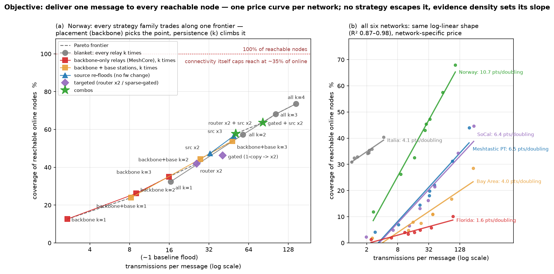
The result is one finding: on a log-airtime axis, every strategy family collapses onto a
single price curve — on Norway roughly eleven points of reachable-node coverage per
doubling of transmissions — and nothing rides above it, while both adaptive rules sit
slightly below it. The collapse itself reproduces on all six networks
(experiment_alltoall_multinet.py: log-linear fit R² 0.87–0.98), but the
slope — the network's airtime-to-coverage exchange rate — is a network
property, ranging from 10.7 points per doubling (Norway) down to 1.6 (Florida) in the same
evidence-density order as Table 4: the sparser the usable link graph, the less any amount
of airtime can buy. The MeshCore pattern is not a better curve but a different point on
the same one:
with Norway's organic role mix (30 backbone nodes) it is the cheapest configuration measured
(2.7 tx per message) at correspondingly low coverage (12.6%); its real-world efficiency
comes from engineered repeater placement, which is topology, not protocol. The same collapse
settles whether broadcast could be folded under GradCor as the special case
dst = everyone: with every node a destination the gradient is zero everywhere, the
corridor admits every receiver and GradCor reduces to managed flood exactly. Unicast
and all-to-all are the two ends of Figure 1's knowledge spectrum and each end is already
at its optimum — corridors cannot help a flood, floods cannot match corridors for a named
destination. What remains is menu pricing per message class (beacons at k=1 and hop limit 7;
higher-value broadcasts one rung up: backbone ×2 or a source re-flood) and the one lever
that moves the whole curve instead of sliding along it: connectivity itself.
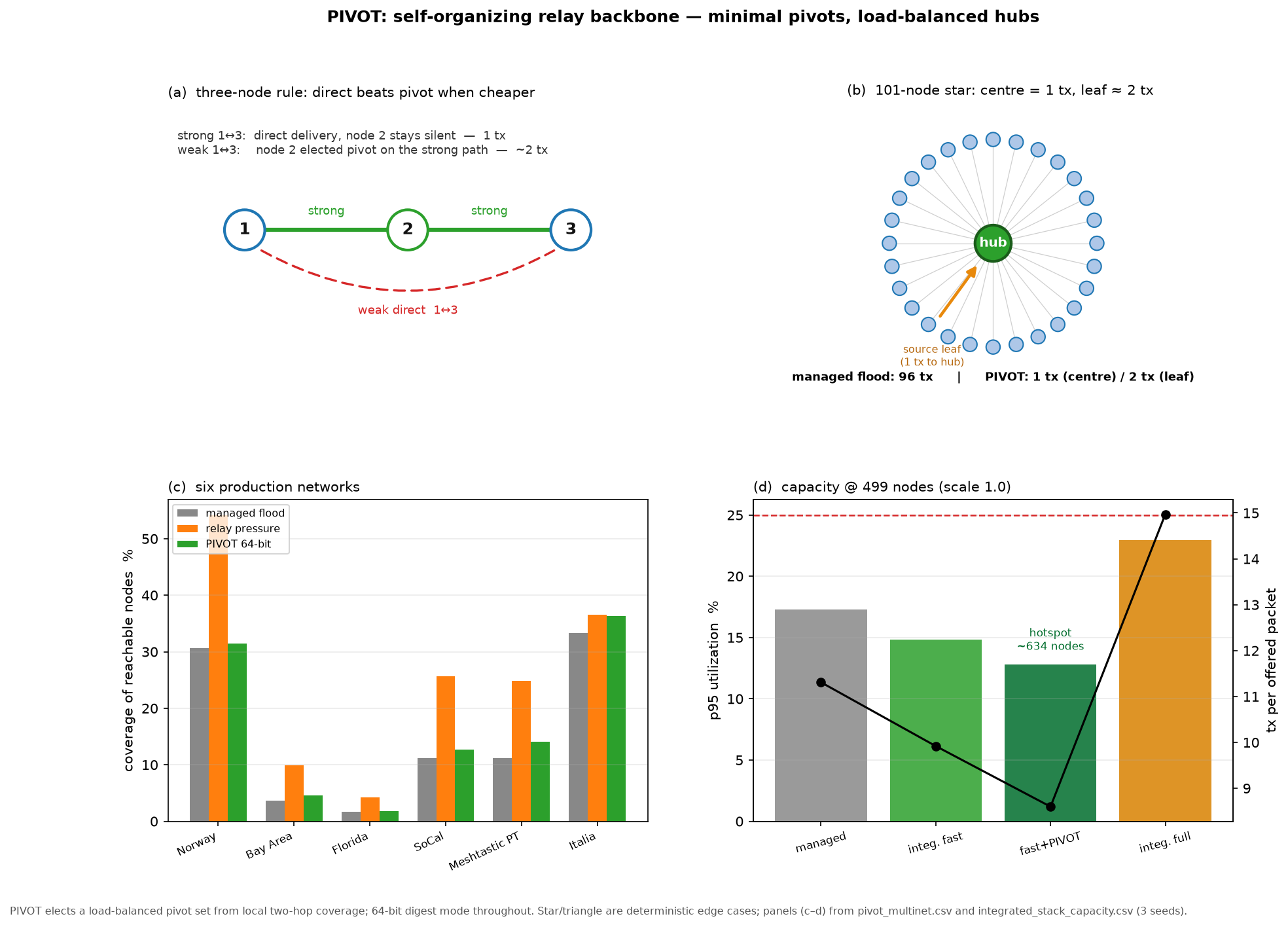
The price curve (§6.4) prices how much redundancy to buy; it does not say who should spend it. Relay pressure (§6.9) answers that per packet from duplicate counts, but it learns only after forwarding and cannot express the star-topology fact that one hub should relay for a hundred leaves. PIVOT (Pivot Relay Backbone) closes that gap with a local two-hop multipoint-relay heuristic adapted from OLSR MPRs: each node learns reliable one-hop neighbours from ordinary traffic; on every broadcast hop it computes which nodes are still uncovered in its two-hop horizon, marks relays that are the only path to any such node as mandatory, then greedily completes the set by greatest residual coverage, tie-breaking on bidirectional ETX, uptime, observed forwarding novelty and remaining channel headroom. Winners receive short relay leases; utilization lowers a hub’s score so load migrates. Non-pivots wait for a pivot echo and relay only if residual coverage stays silent — direct reception always wins.
Two digest modes bracket deployability. PIVOT-exact carries the full covered set (a
simulation ceiling). PIVOT-64/256 replaces it with a k-hash bloom sketch (8 or 32
bytes) in the packet header, charging the byte overhead in every transmission. Edge cases
confirm the rule: a 101-node star costs 1 transmission from the centre and 2 from a
leaf (vs 96 for managed flood); a three-node triangle suppresses the middle node when the
direct link is strong and elects it when direct is weak (100% delivery at ~half the airtime in
both cases, experiment_pivot.py). But the sketch has a hard limit worth stating
plainly: a 64-bit filter saturates once a neighbourhood exceeds a few dozen nodes, and a
saturated filter reports uncovered nodes as covered, so pivots under-relay. On the dense
synthetic world this collapses coverage from 81% (exact) to 33% (64-bit); 256 bits
recovers it to 62% at proportionally more header airtime. This is the honest separation of
algorithmic gain from sketch cost the digest sweep was built to expose: PIVOT’s ceiling
is real, but a byte-bounded firmware sketch only reaches it in sparse neighbourhoods.
That caveat is why the production result is a capacity gain, not a coverage gain. Across six
networks (experiment_pivot_multinet.py; Figure 17) all six are sparse enough
that 64-bit suffices, and there PIVOT does not beat the §6.4 price curve — it
picks a cheaper point on it. On Norway it matches managed-flood coverage
(31.5% vs 30.6% reachable) at similar airtime (14.2 vs 15.4 tx), and sits far below relay
pressure’s 54% coverage — pressure simply buys a more expensive point (59 tx).
The value is capacity, and it is bought with reach: integrated end-to-end
(experiment_integrated_stack.py, PIVOT replacing relay pressure with GradCor-R,
message classes and setpoint unchanged), at today’s mix p95 utilization falls
17.3% → 12.9% and the p99 hotspot warning rises from 445 (managed) to 634
traffic-equivalent nodes (+42%) — but broadcast reach drops from 6.3 to 5.2
receivers per packet (unicast delivery is unchanged, 66.7% vs 66.1%). PIVOT trades
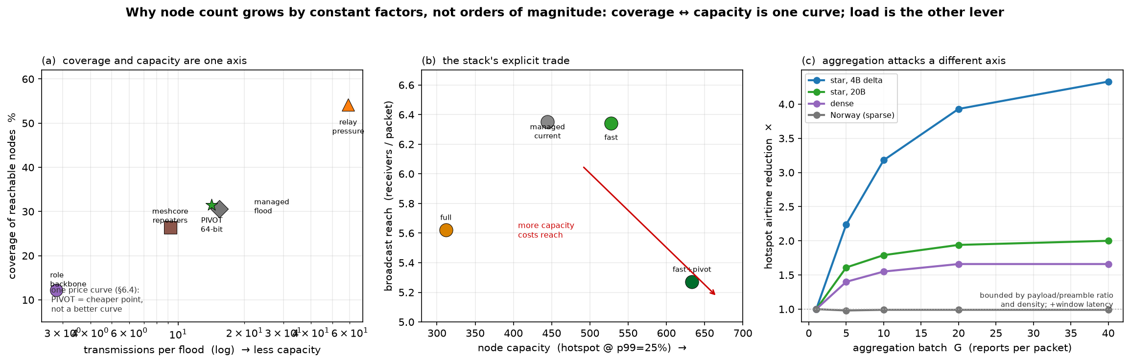
coverage for capacity along the one curve; it does not escape it (Figure 18a,b). PIVOT and
pressure are complementary: pivots are persistent neighbourhood infrastructure, pressure the
packet-local fallback when sketches saturate or topology is too sparse for two-hop summaries.
A pattern now recurs across §6.3–§6.5: PIVOT, relay pressure and the price
curve all reduce transmissions per flooded packet, and each buys a constant factor
— PIVOT ~1.4× airtime on Norway, the whole stack ~1.5×. None of them reduces
the number of packets, yet 79% of the traffic is periodic BULK broadcast (position,
telemetry, NodeInfo) that is inherently aggregatable. That is a second, orthogonal axis: a hub
can collect its neighbours’ reports over a short window and flood one packet
carrying G reports instead of G separate floods (experiment_aggregate.py). We
modelled LoRa time-on-air exactly (Semtech ToA, LongFast-like SF11/BW250) and accounted airtime
per node, because the constraint that caps node count is the busiest node (§6.11),
not the channel total.
The result draws the real boundary on how far software can go. Aggregation cuts the hotspot
node’s airtime, but the win is bounded by two things it cannot change. First, the
payload/preamble ratio: an aggregate of G reports pays one preamble but G payloads, so
with 20-byte reports the ceiling is ~2× (star, hub load 42→21 s at
G≥20) — and it only reaches ~4× if reports shrink to 4-byte deltas, where the
preamble dominates (Figure 18c). This makes the ceiling a moving target in the wrong
direction: per-packet signing and the name-field size changes on the 2.8 roadmap[8] both add
bytes, and every added byte pushes the payload/preamble ratio further from where aggregation
pays. The lever that lifts the ceiling and the lever that authenticates traffic therefore pull
against each other, which is an argument for delta/compressed telemetry encodings rather than
against signing. Second, and decisively, density: aggregation needs
hubs that hear many neighbours. On the dense synthetic world it delivers 1.7× hotspot
relief; on the real, sparse Norway mesh it delivers essentially nothing (0.99×),
because most nodes are their own best hub and batches never fill. Information coverage is
preserved or slightly improved throughout (a receiver of the aggregate gets every report in
it), and the price paid is latency — the window W is added to every report. Production
beacon cadence shows that price is steeper than a window parameter suggests
(experiment_beacon.py): at the measured typical-node telemetry interval, filling a
batch of 20 takes roughly 30 hours in Norway and about four days pooled across the six
networks. Aggregation is therefore a tool for tolerant traffic only, and the batch sizes at
the right-hand end of Figure 18c are not reachable for anything a user waits on.
This is the answer to “why doesn’t node count grow an order of magnitude?” Coverage and capacity are not two goals but two ends of one price curve (Figure 18a): every relay policy slides along it, so more capacity is bought with less reach and vice versa, and the curve’s slope is fixed by physical placement, not protocol. Aggregation is the only lever that moves off that curve, by attacking offered load — but it is capped at a small factor by radio physics and pays out only where the mesh is already dense. The compounding that a large network needs (PIVOT’s ~1.4× × aggregation’s ~2× × the stack’s governors) yields a few-fold headroom, not a decade. An order-of-magnitude increase requires either byte-level change — delta/compressed telemetry that lifts the aggregation ceiling — or spatial reuse: more geography, not more logic on the same spectrum.
A smooth curve offers no natural breakpoints, so any operational split into “message
classes” is a policy quantization — but three empirical facts pin where a small set
of classes should sit. First, temporal repetition rides the same curve: the union
coverage of m successive baseline floods from the same source grows 13.5% (m=1) → 24%
(m=3) → 39% (m=12) — about six points per doubling of cumulative airtime
(experiment_temporal.py), inside the family band of Figure 16. Periodic
traffic — positions, telemetry, NodeInfo, the bulk of a mesh's load — therefore
already climbs the curve by repeating; granting it per-flood redundancy would pay for the same
coverage twice. Second, one step has distinctly best marginal efficiency (backbone ×2:
nine points for +56% airtime, one firmware predicate). Third, returns diminish steeply past
about two doublings (blanket k≥3 spends 100+ transmissions to stay under 75%) —
beyond that is not a class but an emergency action. Three classes, spaced roughly one
airtime-doubling apart, exhaust the useful range (Table 7); finer splits are not
resolvable against seed noise (±0.5–1 point) and would pretend a precision the
network-specific slope (1.6–10.7 points per doubling) cannot honour. The class labels
generalize across networks; the absolute coverage each buys does not.
| Class | Mechanism | Norway point | Default assignment |
|---|---|---|---|
| BULK | k=1, hop limit 7 | 32% per flood, compounding over repeats | periodic broadcasts: position, telemetry, NodeInfo |
| STANDARD | + backbone relays ×2 | ~41% | one-shot human broadcasts: channel texts |
| ASSURED | + source re-flood (×2) | ~58% | alert-class traffic |
Should classes be pre-assigned per message type, or user-selectable? The economics are asymmetric: the class multiplier is paid by the neighbourhood's airtime, not the sender's, so unconstrained user choice is a commons problem. The defensible middle is defaults by port/type (the Table 7 assignment) plus a rate-limited per-node override — a user may pin, say, a critical telemetry stream one class up, within a budget of above-BULK sends per hour; an exhausted budget degrades the sender back to BULK rather than degrading the mesh. Implementation is small: the class fits in two header bits — and can share the field GradCor already uses, since a packet is either unicast (the bits carry corridor level) or broadcast (they carry the redundancy rung), never both — relays act on it locally (backbone doubles at STANDARD and above) and only the source acts on ASSURED's re-flood.
One bias in the replay deserves its own experiment: the link graph is built from hop≤7
traceroutes and all floods obey the wire's hop field, so gradient descent beyond seven hops
is never exercised on real data — the no-hop-limit property of §3 is proven at
the spec level, not stress-tested. We therefore built synthetic “braid” topologies
with three controlled parameters: d, the depth — the true hop distance from
source to destination, which the construction fixes exactly (the source sits in column 0, the
destination in column d, and a packet must cross every column); w, the number of
parallel lanes per column (the receiver diversity anycast feeds on); and p, one
per-transmission delivery probability on every link. Full links connect consecutive columns,
every node is always on, so depth is isolated from churn. We then measured GradCor-R at depths
the replay never sees
(experiment_depth.py; Figure 19).
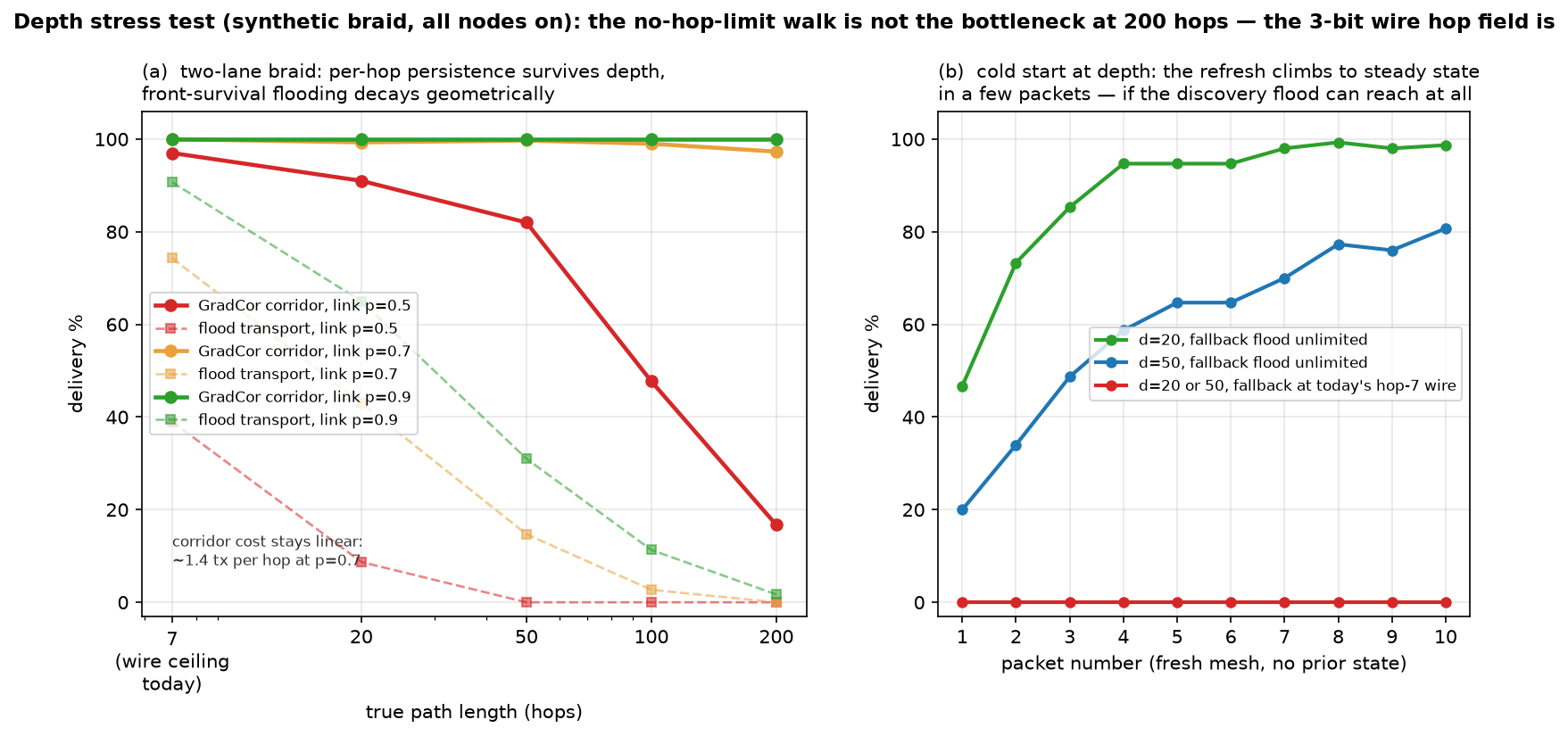
The walk is not the thing that breaks at depth. With warm gradients on a two-lane braid at p = 0.7, delivery is 100% at 7 hops, 99% at 100 and 97% at 200 hops, with cost staying linear at roughly 1.4 transmissions per hop — per-hop anycast persistence (up to five broadcasts across parallel candidates) makes each hop nearly certain, so depth only multiplies cost, not risk. Carrying the same packets by unlimited-hop flood instead decays geometrically — 74% → 43% → 3% → 0% over the same depths — because a flood front gets one trial per link and must survive every stage. The honest failure regime is equally visible: a single chain (w=1) of weak links (p=0.5) collapses at depth (77% → 0%); anycast diversity is the load-bearing ingredient, and GradCor needs some receiver redundancy per hop — which any real mesh dense enough to span 20 hops provides.
Cold start at depth exposes a wall, and it is not GradCor's. With no prior state, the first packet falls back to a discovery flood — and today's 3-bit wire hop field caps that flood at 7, so a fresh 20-hop conversation delivers zero, for every protocol, ours included. Grant the fallback flood unlimited depth and the ramp is quick: at depth d=20 the first packet delivers 47% and packets 4 onward ~95–99% as each success re-stamps true distances; at d=50, 20% ramps to 80% by the tenth packet. The practical reading for deep meshes: the corridor removes the per-packet hop ceiling today, within the existing packet format; extending discovery beyond 7 needs a header change that any 20-hop ambition requires regardless of routing scheme. Caveats: the braid is synthetic and fully awake — it isolates depth, deliberately excluding the churn and asymmetry the Norway replay covers.
And broadcast itself can be fixed the same way the corridor was. The corridor survives
depth because of per-hop persistence, and that mechanism transplants directly into the flood:
let a relay retransmit (up to R times) until it overhears an onward arrival — the
same implicit-ack primitive as the contention race of §3.3 and the managed flood's
overhear-cancellation, with the policy inverted: repeat-until-heard instead of mute-when-heard.
Measured on the same braids (experiment_persist.py; Table 8): today's flood
(R=1) delivers 7.7% of packets to the 200-hop far end at p=0.7; R=3 delivers 100%, at
~2.5 transmissions per relay — geometric decay converted to a linear cost factor, exactly
as in the unicast walk, and even weak links reach 99.7% at R=5. Depth is therefore solved
in mechanism for broadcast too; what remains unsolved is arithmetic: one packet
crossing 200 hops costs ~500 transmissions mesh-wide, fine for a rare alert, catastrophic for
periodic telemetry from every node in a mesh large enough to have such a diameter (O(N)
transmissions per beacon, N beaconing nodes). No forwarding mechanism fixes that; only scoping
does — aggregation at region boundaries, interest-based forwarding toward subscribers
(which quietly turns the traffic back into unicast, where the corridor already operates), or
accepting that beacons are a neighbourhood fact and long-haul telemetry travels to named
collectors. Large networks never flood measurements; they aggregate — this is why.
| Depth | Link p | R=1 (today's flood) | R=3 | R=5 | Tx/packet at R=3 |
|---|---|---|---|---|---|
| 20 hops | 0.7 | 74.3% | 99.3% | 100% | 55 |
| 50 hops | 0.7 | 53.0% | 100% | 100% | 127 |
| 200 hops | 0.7 | 7.7% | 100% | 100% | 487 |
| 200 hops | 0.5 | 0.0% | 88.0% | 99.7% | 572 |
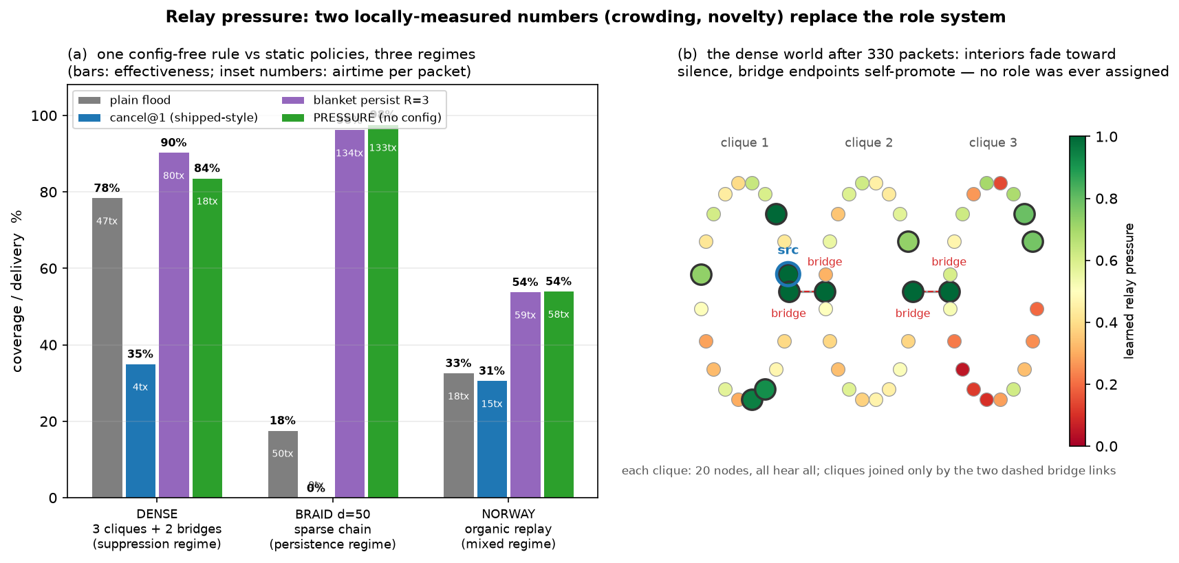
§6.5's PIVOT backbone elects persistent neighbourhood pivots from two-hop coverage; this section tests the complementary per-packet rule that needs no topology summary — useful when digest sketches collide or evidence is too sparse for MPR convergence. Sections 6.3–6.7 leave the flood with a structural tension: the right relay policy is regime-dependent — sparse meshes reward persistence (§6.8), dense neighbourhoods reward suppression (§8, item 4), and a few well-placed nodes carry outsized value (the backbone rungs of Table 6) — yet the mechanism that assigns policy today is a hand-configured role enum, the last piece of human-guessed structure in the system. Physical placement is the constant no protocol can change; everything above it should calibrate itself. We tested whether it can, with the same move GradCor applied to unicast: replace configured structure with evidence the radio already provides. Each node maintains two numbers, both free of control traffic: crowding c, an EWMA of how many duplicate copies of each packet it decodes (“how covered is my neighbourhood without me?”), and novelty, an EWMA of whether its own relays still produce first-copy receivers (“does my transmission create coverage that would not otherwise exist?”). Its relay pressure is the maximum of the two terms, and pressure alone sets the policy ladder: contention slot (high pressure transmits first), cancellation threshold (low pressure mutes on the first overheard relay, high pressure never mutes) and echo-persistence (§6.8's R, from 1 to 3). A node in a crowd fades toward silence unless its transmissions keep reaching someone new — which is precisely the definition of a bridge.
The test is falsifiable and three-legged (experiment_pressure.py; Figure 20,
Table 9): one config-free rule must match the best static policy in every regime,
where each regime's best static differs. It does. On a dense world (three 20-node cliques
joined by two single bridges — the regime where suppression wins) pressure reaches 93%
of the best coverage at a quarter of its airtime, Pareto-dominating the plain flood on
both axes, and the twelve nodes that self-promote to high pressure include all four bridge
endpoints — discovered by passive listening, with no role ever assigned. On the sparse
braid (the regime where persistence wins) it matches blanket persistence, 97.7% vs 96.3% at
equal cost. On the Norway replay it matches the best static policy (54.1% vs 53.9%) —
21 points above today's flood — with every node allowed to relay and no CLIENT_MUTE
configuration consulted. The mechanism also failed informatively along the way: crowding alone
suppresses the bridges together with the crowd (dense coverage collapses to 34%), and an
active variant that probed by occasionally staying silent learned too slowly; the signal that
works is passive outbound novelty. Caveats mirror the section's others: the simulator observes
first-copy receptions directly, while firmware must infer novelty from onward relays and acks
— under-crediting nodes that serve silent leaves is the design problem to solve in a
port — and the dense world's slotted contention model is still gentler than a truly
congested channel, which is the regime where suppression's value should grow further.
| World (regime) | Best static policy | Best static | Pressure (no config) |
|---|---|---|---|
| Dense: cliques + bridges (suppression) | blanket persist R=3 | 90.4% @ 80.0 tx | 83.7% @ 18.4 tx |
| Braid d=50 (persistence) | blanket persist R=3 | 96.3% @ 134.0 tx | 97.7% @ 133.2 tx |
| Norway replay (mixed) | blanket persist R=3 | 53.9% @ 59.0 tx | 54.1% @ 58.3 tx |
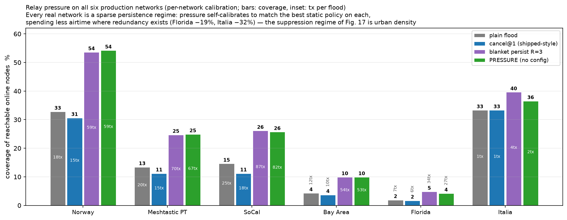
Running the same head-to-head on all six production networks
(experiment_pressure_multinet.py; Figure 21) adds the cross-network check:
pressure matches the best static policy on every network — which is persistence on all
six, since every evidence-sparse organic mesh is a persistence regime — while spending
less airtime wherever local redundancy exists (Florida −19%, Italia −32%). The six
real networks therefore validate the rule's safety, not its full range: none of them is dense
enough to exercise the suppression side, which is exactly the urban regime Figure 20's
synthetic dense world covers and the regime a firmware trial in a city core would test
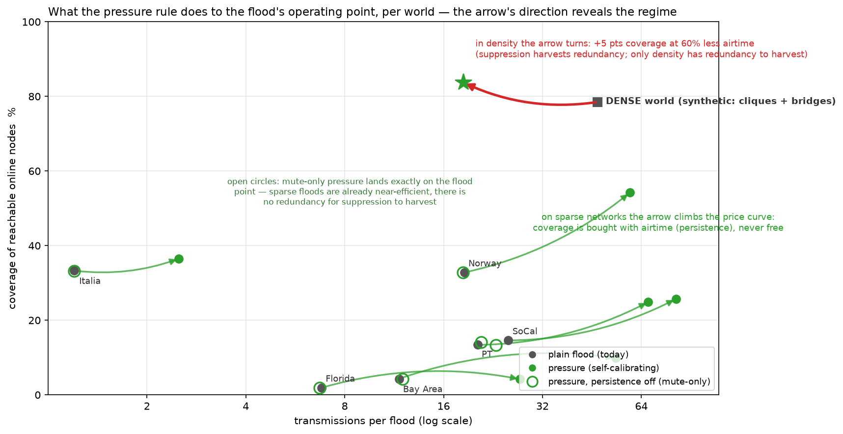
first. A persistence-only-off variant sharpens the boundary: with muting as the only lever,
pressure reproduces plain flood's coverage and airtime almost exactly on all six networks
(Norway 32.8% at 18.3 tx vs 32.8% at 18.5) — sparse floods are already
near-efficient, because suppression can only harvest redundancy and sparse meshes have almost
none. The airtime dividend lives in density, where pressure collects it automatically.
Two governors bound the rule in deployment. First, pressure composes with the message classes of §6.7: pressure decides who relays and with what priority, the class caps how much persistence a packet may buy (BULK at R=1 — periodic traffic is already self-redundant, §6.7 — STANDARD at 2, ASSURED at 3), so the multi-fold airtime of full persistence is spent only on traffic that warrants it. Second, an airtime governor makes “best effort without breach” self-calibrating rather than configured: the two required signals — the node's own duty-cycle spend and observed channel utilization — are already measured by the firmware for regulatory accounting, and effective persistence is simply Reff = min(Rpressure, Rclass, Rbudget), where Rbudget derates toward 1 as either signal approaches its ceiling. The hard budget guarantees regulatory compliance; the surplus, where it exists, is spent exactly where pressure says it buys coverage. No user knob is required — and none should be offered, since the airtime being spent is the neighbourhood's, not the sender's (§6.7). Figure 22 compresses the whole trade into one view: the direction the pressure rule moves each world's operating point reveals its regime.
The message-class and pressure governors above only derate near breach. The full form of the idea is a
bidirectional controller: since the price curve (§6.4) is a menu, no node should pick one
point on it forever — it should slide along it with the channel's current state,
spending surplus airtime on coverage when the medium is idle and retreating below plain flood
as it fills. The signal is again one the firmware already measures: local channel utilization
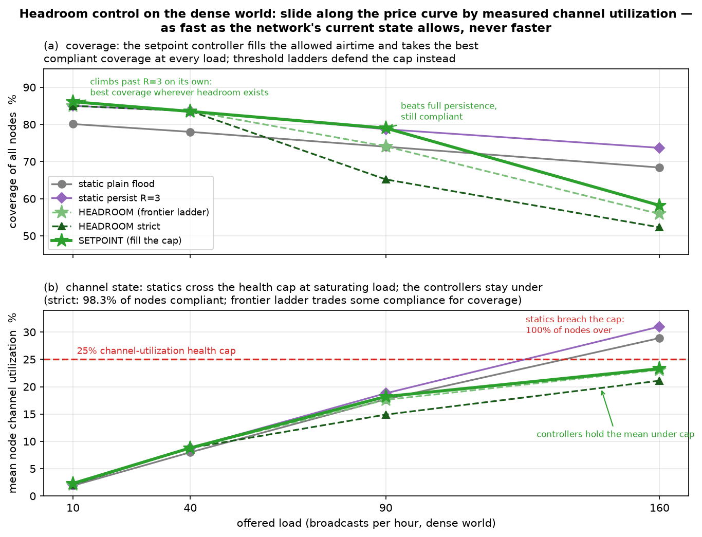
u. The controller tested here is three thresholds referenced to the 25% community health cap
— u < 18%: full persistence, never cancel (top of the curve);
u < 24%: R=2, cancel after two echoes; beyond: R=1, cancel on the first echo
(below plain flood). For the test to be fair, congestion must cost something, so reception in
this experiment suffers utilization-coupled interference (extra loss
min(0.6, 0.8u)); offered load is then swept from quiet to saturating on the dense world
(experiment_headroom.py; Figure 23, Table 10).
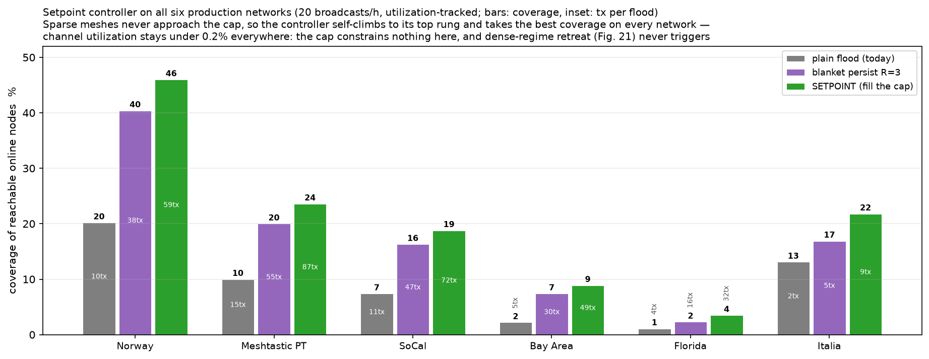
The controller does what it promises, and its first version taught a design lesson worth recording. At idle both versions are indistinguishable from the best static policy — the surplus is spent, nothing is left on the table. The lesson emerged at moderate load: our first ladder retreated from full persistence to (R=2, cancel after two echoes), coupling every persistence reduction with more cancellation — and since cancellation starves bridge feeding, that ladder skipped the plain flood's operating point entirely, covering 65% at a load where plain flood managed 74%. The corrected ladder descends through the Pareto frontier — full persistence → plain flood (R=1, never cancel) → emergency cancel@1 — and at moderate load matches plain flood's coverage exactly (74.1%) while staying compliant. At saturating load the trade becomes genuine and no ladder abolishes it: every static policy breaches the health cap (plain flood included: 29% mean utilization, 100% of nodes over), and the controller must choose what to protect — the frontier ladder preserves more coverage (55.9%) at partial compliance, the strict (cancellation-coupled) ladder enforces the cap almost perfectly (98.3% of nodes under) at 52.3%. Cap strictness is thus the one genuine policy choice in the stack; everything else self-calibrates. Two further disclosures: on the sparse production networks the controller is a no-op — even 120 broadcasts per hour cannot push Norway past 0.7% utilization, so it sits at full persistence permanently — and the thresholds needed one referencing pass against the cap.
The completed form of the idea inverts the framing once more: do not defend the cap, fill it. The setpoint controller drops thresholds entirely — each node hill-climbs a rung ladder ordered by airtime appetite (emergency → plain flood → persist R=2…5), climbing while its measured utilization sits below 80% of a target just under the cap and descending above it. Coverage is then whatever the allowed airtime buys, and it matches or beats every static and every threshold ladder at every load (Table 10, last column): above the best static at idle (86.1% vs 85.0%, having climbed past R=3 on its own), above full persistence at moderate load while compliant (79.0% vs 78.7%, where plain flood manages 74.0%), and the best compliant coverage at saturation (58.2%). One honest caveat: a cap-filler is optimal for “maximize coverage subject to u ≤ cap,” not per-transmission efficiency — at idle it spends 30% more airtime than persist R=3 for one extra point, because the price curve's diminishing returns are invisible to a controller that only watches utilization; a deployment wanting frugality would add a marginal-gain floor. With this, the governor stack is complete: pressure decides who relays (topology), class decides how much a packet may buy (value), headroom/setpoint decides how much the channel can afford right now (state) — three dials, three already-measured signals, zero user knobs.
| Load (floods/h) | Persist R=3 | Plain flood | Headroom (frontier ladder) | Headroom strict | Setpoint (fill the cap) |
|---|---|---|---|---|---|
| 10 | 85.0% @ 72 tx, u=2% | 80.1% @ 48 tx, u=2% | 85.0% @ 72 tx | 85.0% @ 72 tx | 86.1% @ 94 tx |
| 40 | 83.6% @ 68 tx, u=9% | 78.0% @ 47 tx, u=8% | 83.6% @ 68 tx | 83.6% @ 68 tx | 83.5% @ 85 tx |
| 90 | 78.7% @ 64 tx, u=19% | 74.0% @ 44 tx, u=18% | 74.1% @ 49 tx, u=18% | 65.2% @ 46 tx, u=15% | 79.0% @ 80 tx, u=18% |
| 160 | 73.7% @ 63 tx, all nodes over cap | 68.4% @ 41 tx, all nodes over cap | 55.9% @ 20 tx, 67% over | 52.3% @ 24 tx, 1.7% over | 58.2% @ 27 tx, 67% over |
Cross-network validation closes the section (experiment_setpoint_multinet.py;
Figure 24): on all six production networks, under the same utilization-tracked harness,
the setpoint controller takes the best coverage on every network — Norway 46.0% vs the
best static's 40.4%, and ahead on all five others — while utilization never exceeds
0.2% anywhere: sparse meshes cannot approach the cap, so the controller correctly never
retreats and simply spends the abundant headroom. The same caveat scales with it: the top
rungs buy those extra points at steep marginal cost (Norway: +5.6 points for +57% airtime),
which is optimal against the cap objective and wasteful against a frugality objective —
the choice of objective, like cap strictness, is the deployment's one real decision.
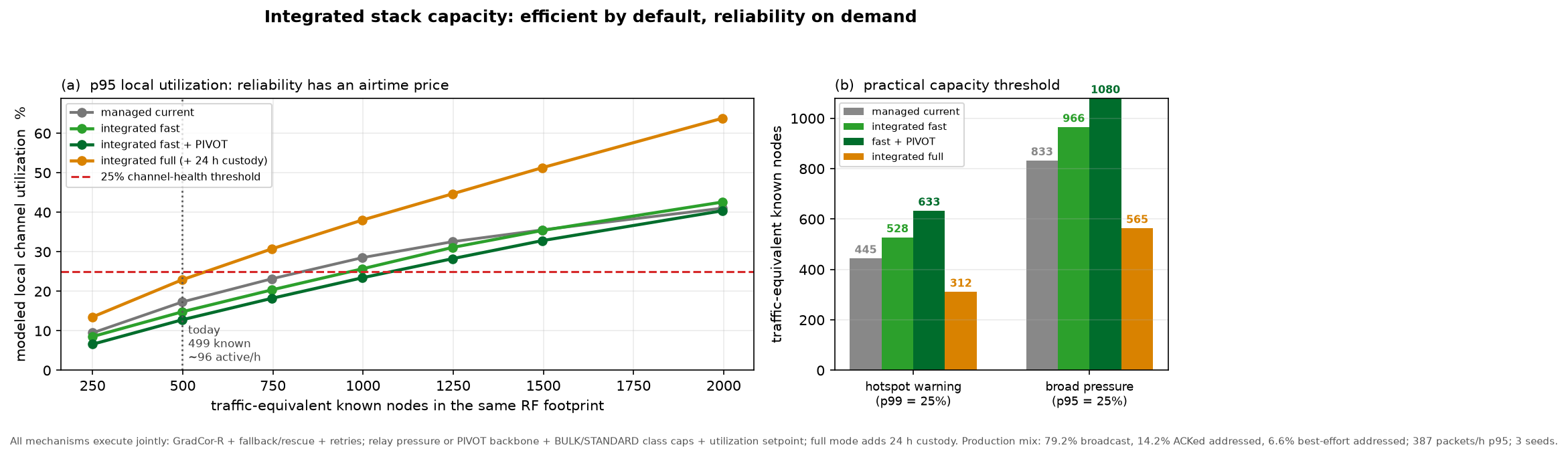
Node count alone has no physical limit: what fills the channel is airtime within one
interference neighbourhood, so geographic expansion can add nodes while reusing the same
spectrum elsewhere. A useful Norway-specific answer must therefore hold the RF footprint and
per-node behaviour fixed. We deduplicated the study week's production rows by canonical
(source_node_id, packet_id): 51,892 packets, 309 per hour on average and 387 in
the p95 hour, from 96.1 active sources per hour among 499 known nodes; 79.2% were broadcast.
The integrated replay (experiment_integrated_stack.py) fixes the calibrated
Norway topology and presence trace, multiplies that p95 offered load, and reports the
multiplier as “traffic-equivalent nodes.” It preserves the canonical packet mix:
78.93% BULK broadcast, 0.25% STANDARD broadcast, 14.17% want_ack addressed and
6.65% best-effort addressed. Managed current floods both kinds and gives ACKed traffic
three end-to-end retries. Integrated fast executes the stack jointly: relay pressure (or PIVOT backbone in the
fast+PIVOT variant), message-class caps and the utilization setpoint govern broadcast; GradCor-R with
fallback-flood cold start, local rescue and the same ACK retries carries addressed traffic.
Integrated full adds the final reliability-envelope step: failed ACKed packets enter
24-hour custody and retry hourly when both endpoints are online. Identical event schedules run
for three seeds; 0.5 s transmissions feed the utilization-coupled loss proxy of
§6.11. Thus every box in Figure 28 executes, but the reliability envelope is measured
as an optional operating mode rather than assumed free.
At today's 499-node equivalent, integrated fast+PIVOT is the capacity winner: transmissions per offered packet fall 11.3 → 8.7, p95 utilization 17.3% → 12.9% and p99 27.8% → 20.1%, while unicast delivery rises 41.0% → 66.7% (vs 66.1% for integrated-fast without PIVOT). Its p99 hotspot warning moves from 445 to 634 traffic-equivalent known nodes (+42%), and its p95 broad-pressure point from 833 to 1079 (+30%). Integrated-fast without PIVOT still beats managed current (+19% / +16%) but leaves broadcast airtime on the table. Integrated-full raises unicast delivery again to 79.1%, but costs 15.0 transmissions per offered packet and moves the two capacity thresholds inward to 312 / 565 nodes. Custody is doing its job — spending later airtime on packets the present topology could not carry — but that makes the design rule empirical rather than stylistic: the fast+PIVOT stack is the default; 24-hour custody belongs only to rate-limited ASSURED traffic. Turning it on for every ACKed exchange converts reliability into congestion. For this footprint the operational fast-mode answer is therefore ~630 nodes as the local warning and ~1080 as broadly loaded, not a universal Meshtastic ceiling; geographic spread can reuse airtime, while denser overlap or bursty traffic lowers the bound.
Review of this work by a Meshtastic maintainer identified three places where the result leaned on something assumed rather than something observed: that anycast contention suppression works on real radios; that a mesh cycles duty rather than moves, which is what justified deleting the state clocks; and that the delivery half of the headline belonged to GradCor rather than to the reliability envelope around it. All three are now measured. Two came out in the paper's favour by a wider margin than expected. The third was a fair hit, and correcting it produces a stronger claim than the one it replaces.
Contention suppression is not load-bearing, because the corridor is narrow. Every result
above charges one transmission per forwarding decision: the lowest-gradient candidate takes the
packet and every other eligible receiver hears it and stays silent. If a loser fails to hear the
winner it transmits anyway, so this assumption sits underneath every airtime number in the
paper. The first thing to measure is not whether suppression works but how often it is needed:
across 165,430 forwarding decisions the mean contention set is 1.38 candidates and
63.2% of decisions have no loser at all. Strict gradient descent is its own admission
control, and it has already discarded most of the neighbourhood before any timer runs.
Relaxing the assumption confirms what that geometry implies
(experiment_suppression.py, Figure 26a). Whether a loser hears the winner need
not be a free parameter — both are nodes in the reconstructed topology, so a loser can be
made to suppress only when it actually receives the winner's transmission over the same fitted
link probabilities as everything else. That graph-derived floor is brutal, and deliberately so:
traceroutes only record links that carried traffic, so loser←winner edges are mostly
unobserved and the model concludes that just 9.5% of suppressions succeed — far
worse than any real radio neighbourhood, where candidates sharing a transmitter are usually
within earshot of each other. Even there GradCor-R costs 57.8 transmissions per delivered packet
against flood's 70.8. Forcing suppression to fail outright, on every decision, gives 61.5.
There is no break-even: the airtime advantage degrades smoothly from 3.3× to 1.15×
and never inverts, because a suppression failure converts the walk into a
gradient-restricted flood rather than an ordinary one. Delivery is unaffected throughout
(48–51% at every failure rate), since redundant forwarders add path diversity as fast as
they add cost. Contention timing therefore sets where in that range the protocol lands; it does
not decide whether the claim holds.
The mesh does not move. Deleting wall-clock aging (§3.6) was justified on the
grounds that this network cycles duty rather than moves, and Figure 5's caption concedes
that a high-mobility mesh could recover the clock's value. Both halves of that were assertion.
Production position packets settle it, though the measurement is mostly data-quality work
(experiment_mobility.py). Meshtastic lets a node broadcast a deliberately imprecise
position, and the most common setting in production, precision_bits = 13,
quantizes to a ~5.8 km grid — a stationary node on that setting manufactures
kilometres of phantom movement. Positions at (0, 0) recur when a node has no fix, and so do
positions at (0.0262, 0.0262), which is exactly (0, 0) after the 13-bit centring
offset. A minority of nodes emit occasional antipodal garbage while sitting still, which
destroys any maximum- or p95-based radius. The robust statistic is therefore r50, the median
distance from a node's own median position, computed only on exact-precision nodes with the
origin excluded. Across all six networks and 1,381 such nodes, 91.5% never move —
80.3% report the byte-identical coordinate every time — 5.0% stay within a kilometre, and
3.5% roam (Figure 26b). Only 3.2% are in motion while reporting, at a median
sustained 27 km/h. The obvious objection is self-selection: privacy-conscious users who
reduce precision might be the mobile ones. That is testable, because a 1.5 km grid still
resolves a 5 km move. Reduced-precision nodes do roam more — 3.90% against 1.76%
past 5 km, a 2.2× bias in exactly the predicted direction — and folding
every precision class together gives a population-wide roaming rate of 3.2% of 5,289
nodes. The bias is real, it has been quantified, and the conclusion survives it.
Even where the mesh does move, the clock does not help — and neither does anticipating
motion. A measured 3% is not an answer on its own, because the mechanism in question is
about what happens when nodes do move: age anticipates staleness, whereas per-hop
escalation only discovers it after a transmission fails. So mobility is swept from 0 to 100% of
nodes relocating roughly every two hours, with each variant given a private world driven by an
identical relocation schedule so the comparison is properly paired across 30 seeds
(experiment_mobility_sim.py, Figure 26c; per-seed results and paired bootstrap
intervals in mobility_ci.csv). Relocation is local drift — a
mover adopts the neighbourhood of a node two hops away, which is what driving through a mesh
looks like. The clock-free variant is significantly ahead of the age-widened one at every
level from 0 to 50% mobility — paired gaps of 1.0 to 1.6 delivery points, every 95%
confidence interval excluding zero — and statistically tied at total churn (−0.10
points, 95% CI [−0.22, +0.02], p=0.23). The anticipated crossover never arrives: at no
mobility level does the clock overtake. The
reason is a timescale the original argument had backwards: escalation is not the slow mechanism
here. It reacts within a single packet's walk, at the hop where the stale entry actually
misleads; a three-hour widening threshold reacts in hours, and reacts identically whether
anything changed or not. Reactive correction is the faster adaptation, not the lazier one.
That result suggested a mechanism worth trying, and it failed instructively. A node that relocates knows it relocated — it carries the GPS or IMU that detected the move — so it can invalidate its own gradient entries at the instant they become wrong. This is anticipation without a clock: event-driven, zero airtime, firing exactly when staleness is created. It should have been the best of both. Instead it is indistinguishable from plain GradCor-R at the measured 3% rate (−0.74 points, 95% CI [−1.64, +0.16]) and clearly worse once mobility rises — −3.5 points at both 25% and 50% — with or without a re-plant beacon. It wins at no level tested. The explanation generalises past this protocol: after a local drift the mover's old distance estimate is usually still approximately right, so invalidating it discards information that was mostly still true and forces a costly replant, whereas keeping it and letting escalation correct it pays one extra transmission only at the hop where it is actually wrong. Both anticipatory mechanisms lose to reactive correction for the same reason — anticipation throws away partially-valid state, while reaction pays only at the point of real failure. We report this because it is the strongest available argument for the clock-free design, and it is an argument we did not expect to be making.
The delivery claim needed restating, and the restatement is stronger. The original
headline pairs two numbers from one operating point: GradCor-R delivers 50.7% where flood
delivers 25.3%, at 3.3× less airtime per delivered packet. The airtime half is
like-for-like. The delivery half is more fragile than it looks, because §6.2 shows most of
the remaining gap to the ceiling closing with end-to-end retries — machinery that is not
GradCor's, that Meshtastic's reliable-delivery layer already has, and that the headline
evaluation denied to every protocol equally (§8, item 8). If retries lift flooding just as
much, "double the delivery" describes the envelope rather than path selection. Giving every
protocol the identical retry budget settles it (experiment_matched.py,
Figure 26d). Retries do lift flooding hard — from 24.7% to 61.3% at k=5, which
is the honest part of the objection — but they lift it along a much more expensive curve,
and the two protocols never touch. Read at matched budgets, on one axis at a time:
| Matched at | FLOOD | NEXTHOP | GRADCOR-R |
|---|---|---|---|
| Delivery at flood's own offered load (17.9 tx/pkt) | 24.7% | 30.7% | 68.4% |
| Delivery at flood's k=5 load (63.7 tx/pkt) | 61.3% | 64.2% | 84.2% |
| Offered load to reach flood's best delivery (61.3%) | 63.7 | 55.6 | 14.9 |
At the airtime managed flooding already spends, GradCor-R delivers 2.8× what flooding delivers; to reach flooding's best delivery it spends 4.3× less airtime. Those replace "double the delivery at 3.3× less airtime" everywhere it appeared. They are larger numbers, but the reason to prefer them is not that they are larger: it is that each fixes one axis and varies the other, so neither can be read as crediting GradCor with a gain the retry envelope supplied.
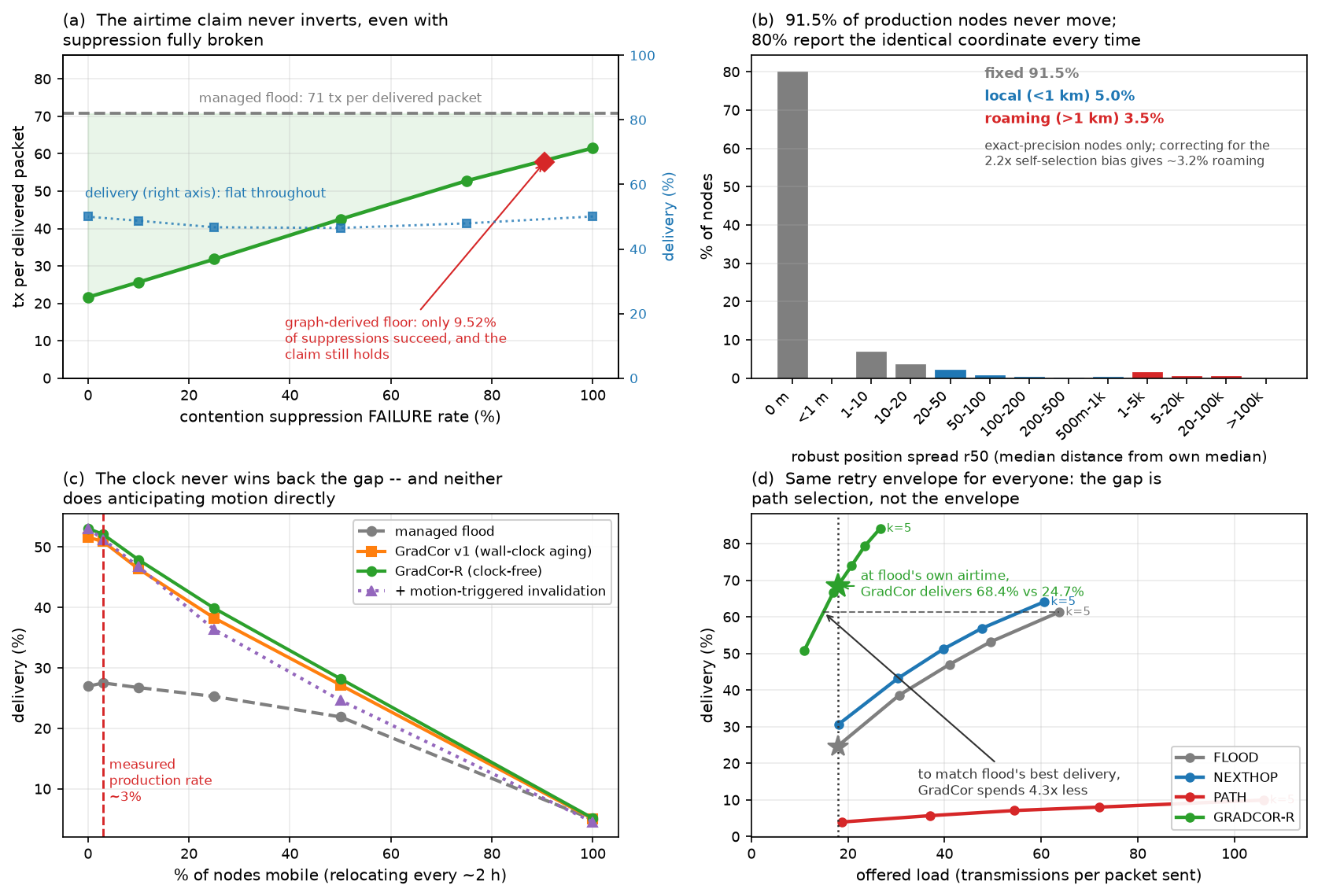
§6.12 tested three assumptions the reviewer named. Auditing our own method afterwards surfaced a fourth that nobody had raised and that turned out to matter more than any of them: the traffic. §5.6's replay has every active pair sending one packet per hour. That number was never measured; it was chosen to give each protocol a workload dense enough to exercise state. Since GradCor's central claim is that state stays fresh because people are talking, a metronome that guarantees hourly talking is not a neutral choice — it assumes the conclusion.
Production addressed traffic is roughly two orders of magnitude sparser than the replay
assumed. Extracting 30 days of addressed packets across all six networks
(experiment_traffic.py) gives 0.261 packets per pair per day on Norway and 0.112
pooled, against the metronome's 24 — a factor of 92 and 215 respectively. The shape is
worse than the rate: 43% of Norwegian pairs and 63% of pairs overall send exactly one packet
in 30 days, the median gap between consecutive packets is 7.0 hours, 34% of gaps exceed
a day, and only 19% of ordered pairs ever see reverse traffic. For most pairs there is no second
packet for a delivery refresh to ride. Two side findings are worth recording: MQTT
gateway duplication is 5.91× on addressed traffic and 11.65× on broadcast, ranging
from 1.12× in Portugal to 31.8× in the Bay Area, so any per-packet rate computed
without deduplicating on (network, source, packet_id) is wrong by a
network-dependent factor; and addressed traffic is overwhelmingly infrastructure rather than
chat — 53.9% NodeInfo, 14.3% traceroute, 4.6% routing ACK, and 0.1% visible text. The
§6.11 capacity work assumed a 79.2/20.8 broadcast/addressed split; measured, it is
76.6/23.4, which holds.
The mesh does, however, beacon constantly — and that is what actually plants
gradients. §3.2's second planting path costs nothing because it rides broadcasts the
destination already sends. Measuring their cadence (experiment_beacon.py) puts the
median gap between a typical Norwegian node's own broadcasts at 59 minutes, and two
to three hours pooled across six networks depending on how aggressively thinly-observed nodes
are filtered (Portugal and SoCal worst, at three hours or more); 51% of Norwegian
nodes broadcast at least hourly and 78% at least three-hourly. NodeInfo clusters exactly on the
firmware's 3-hour default, which is the point: this cadence is a firmware constant, not user
behaviour. These are upper bounds, since a beacon no gateway heard looks like a longer gap, so
the true cadence is faster and the figures below are conservative. The same extraction validates
this paper's cost currency: time-on-air shares computed from real payload sizes track packet
shares closely (position 46% vs 44%, telemetry 26% vs 24%, NodeInfo 19% vs 23%), so counting
transmissions does not misrepresent airtime on this traffic mix.
An external check on the simulator, which the paper previously lacked. Routing ACKs
cannot ground-truth delivery — that table is a 12% decoder subset, observes under 1% of
deliveries we can confirm by other means, and contains no joinable rows at all for Norway's
calibration week. But where the destination is itself an MQTT gateway, its reception is
observed directly. On that subset Norway delivers 26.7% over 30 days and 29.9% on
calibration-week traceroutes, against the model's 25.3% for flooding
(experiment_ack.py). Same universe, marginally pessimistic against a subset biased
toward powered, well-sited destinations — the direction one would want. It does not
license a claim that production delivery is 25%: per-network rates run from 8.4% in
Portugal to 54% in SoCal, and the six-network aggregate landing near 25% is coincidence.
Re-running the comparison on the measured process moves the explanation, not the
direction. Replacing the metronome with the fitted generator and sweeping the beacon
interval B (experiment_realtraffic.py, 200 seeds, Figure 27a) separates the two
free-planting mechanisms cleanly, because flooding and next-hop caching do not use gradients and
so are unaffected by B:
| Beacon interval B | FLOOD | NEXTHOP | GRADCOR-R | R cold starts | R airtime vs flood |
|---|---|---|---|---|---|
| none (conversation only) | 21.7% | 25.0% | 21.9% | 69.7% | 1.34× |
| 24 h | 21.7% | 25.0% | 28.7% | 54.7% | 1.89× |
| 6 h | 21.7% | 25.0% | 34.4% | 39.9% | 2.27× |
| 3 h (pooled measured) | 21.7% | 25.0% | 37.0% | 34.2% | 2.48× |
| 1 h (Norway measured) | 21.7% | 25.0% | 39.8% | 24.5% | 2.57× |
| 0.5 h | 21.7% | 25.0% | 40.5% | 21.4% | 2.60× |
The reading is unambiguous. With conversation alone and no beacons at all, GradCor-R ties flooding (21.9% vs 21.7%) and loses to next-hop caching; seven in ten sends have no usable gradient. Delivery then rises monotonically with beacon frequency to 40.5%. The mechanism that makes GradCor work is ambient broadcast planting, not conversational refresh — the opposite emphasis to the one §3.5 originally gave, and an artifact of the metronome, which was quietly supplying about 90 follow-on packets per pair per week for the delivery refresh to ride. We state this plainly because the corrected mechanism is the more useful claim: it is falsifiable, it identifies a firmware constant as the protocol's operating parameter, and it predicts that meshes which beacon faster benefit more.
At the measured cadence the headline survives, reduced. Re-running §6.12's matched
retry envelope on the real process (experiment_matched_real.py, 30,191 attempts per
arm — matched to the original study's 30,190, Figure 27b) gives:
| Matched reading | Metronome (§6.12) | Norway, B=1 h | Pooled, B=3 h | No beacons |
|---|---|---|---|---|
| Delivery at flooding's own offered load | 2.8× | 2.27× | 2.08× | 1.35× |
| Airtime to reach flooding's best delivery | 4.3× less | 3.14× less | 2.69× less | 1.67× less |
So the paper's headline pair loses roughly a fifth of its delivery advantage and a quarter of its airtime advantage, and keeps the qualitative claim: at the airtime managed flooding already spends, GradCor-R delivers about 2.3× as much, and to match flooding's best delivery it spends about 3.1× less airtime. One sensitivity bounds this from the other side. If beacon airtime is charged to GradCor rather than treated as ambient, the delivery-at-equal-airtime reading is essentially unchanged (2.3×) but the airtime-at-equal-delivery reading collapses to 1.01×. We report the ambient convention as primary because those broadcasts exist in the mesh whether or not the routing protocol changes, and because flooding is charged identically — but a deployment that had to add beaconing to get this cadence would find the airtime case, though not the delivery case, disappears. Norway does not have to add it; it already beacons hourly.
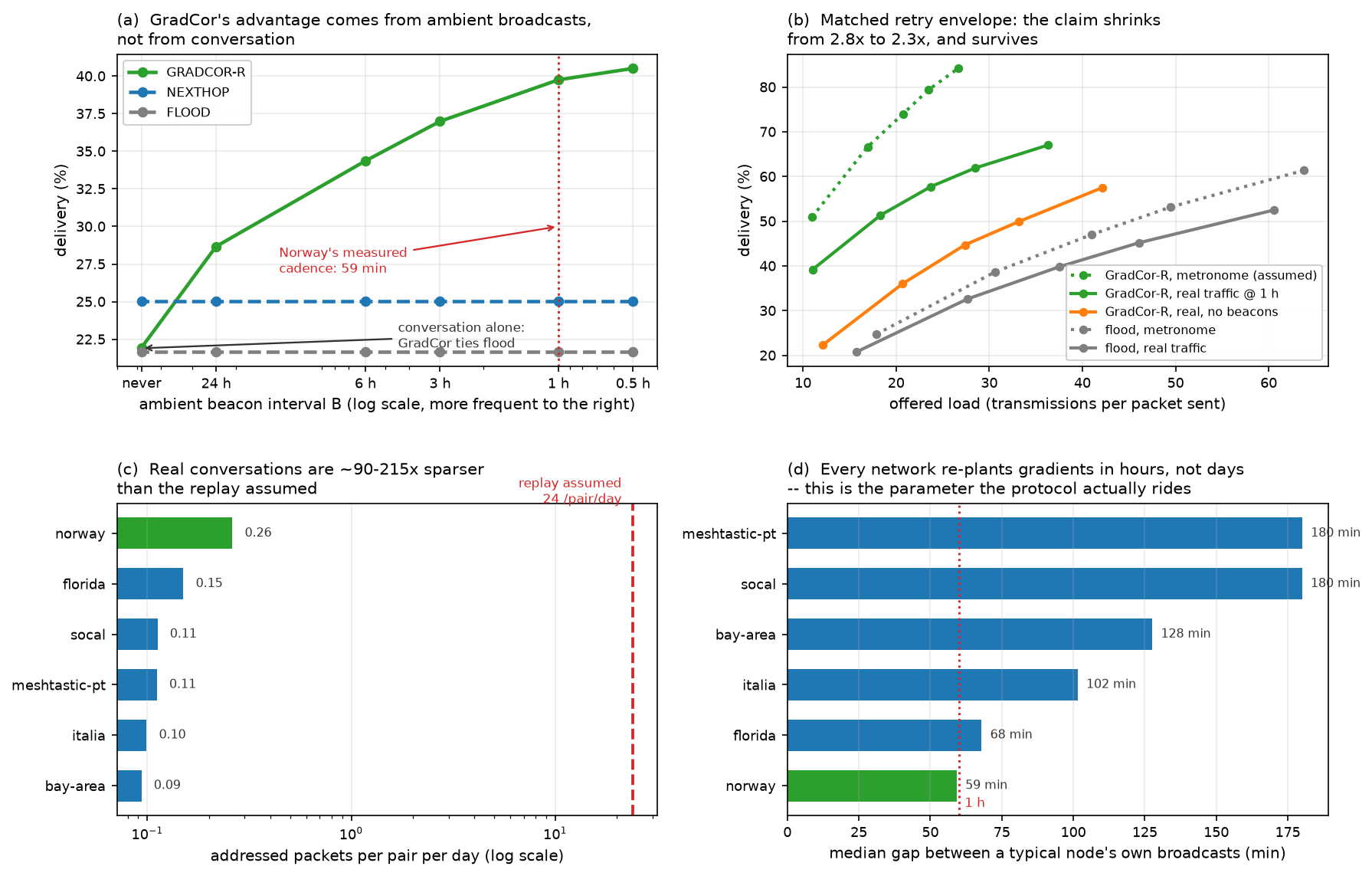
The real topology strengthens the synthetic result. On the synthetic mesh GradCor matched flood's delivery at 2.5–3× less airtime; on the real Norwegian mesh — sparser and harsher than the naive extraction suggested — GradCor-R doubles flood's delivery while keeping the airtime ratio. The mechanism is visible in the graph structure: the ROUTER backbone (degree 53–107 hubs) is present nearly 24/7, so gradients through it stay valid for many hours, while anycast forwarding exploits the receiver diversity that broadcast gives for free — any of several hub-adjacent nodes can carry the packet downhill, so no single lossy link is load-bearing. Notably, the corrected (sparser) graph widened the margin: when links are scarce and marginal, spending them precisely matters more. And the head-to-head confirms the evolution claim in vivo: the clock-free final spec runs even with — here slightly ahead of — the age-widened original (50.7% vs 48.6% at equal cost), with two fewer constants and half the state.
Source routing fails for a measurable, structural reason. PATH needs every hop of a recorded path to work in the named direction and needs the reverse path to deliver the route reply. With 43% of links lacking any working reverse and median 3–4 hop paths, the probability that a full source route remains valid is small and each failure triggers a discovery flood plus a reply that often dies on an asymmetric link. Its 473 tx per delivered packet is worse than never routing at all. This is the algorithm stripped of MeshCore's real-world advantage — deployments built around fixed elevated repeaters with engineered symmetric links — so it should be read as “source routing on an organic mesh,” not as a verdict on MeshCore in its intended setting.
Next-hop caching under-delivers under duty-cycle churn. NEXTHOP edges out flooding (30.4% vs 25.3% at slightly lower cost) but captures little of GradCor's gain: with the median node online 13% of the time, per-destination caches go stale between conversations and most packets fall back to the teaching flood anyway. Its one virtue — zero control traffic and trivial state — remains, which is presumably why Meshtastic 2.6 shipped it. The comparison is to 2.6 as shipped during the study week: the 2.8 line extends the NodeDB address list for next hop[8], and a richer cache would raise this baseline — though not, we expect, the churn that causes its staleness, which is a property of the duty cycle rather than of the table.
Production findings. Building the replay surfaced two extraction defects in the
production topology builder, one of them substantial. First, it parsed traceroute
responses as requests, misorienting their edges and inventing endpoint hops from
mid-flight rows: the corrected extraction shrinks the Norway graph from 3,613 to 1,423 directed
links and raises measured reciprocity from 36% to 57% — meaning the old graph both
overstated connectivity and overstated asymmetry, distorting any coverage, bridge, or
role-recommendation rule computed on it. Second, it discarded route_back/
snr_back, which contribute ~21% of real links and the only direct per-link
bidirectionality evidence — the single most decision-relevant link property for any
routing improvement. Both defects were fixed and shipped to production during this work;
because topology windows are ephemeral and rebuilt from raw rows, every subsequent build
self-heals with no data migration.
Concurrent work: the firmware is already moving this way. The central claim of §6.5, §6.9 and §6.10 — that fixed, hand-set broadcast parameters should be replaced by values a node derives from what it measures — is not ours alone. The 2.8 roadmap carries an item for automatic variable hop limits based on mesh activity and size estimation, explicitly on an empirical or simulated basis, with the rule that the more nodes a sender influences the less often it should send[8]. That is the same thesis arriving independently, and it matters for how this paper should be read in two ways. First, it strengthens the framing: our §6.3 result that the shipped hop limit is the costly setting, and our relay-pressure and setpoint controllers, are not proposals against the grain of the project but arguments for a direction it is already taking — which lowers the adoption barrier the Reddit and Discord responses worried about. Second, it bounds our novelty honestly: adaptive broadcast control is now contested ground, and what remains distinctive here is the unicast side — the one-byte gradient corridor with no hop limit (§3) — together with the finding that adaptive relaying slides along a fixed price curve rather than beating it (§6.6). Those two claims are orthogonal to a variable hop limit: a mesh-size estimate changes where on the curve broadcast sits, not the curve, and GradCor's termination argument never consults a hop counter at all. The natural comparison for future work is therefore direct: measure a mesh-size-estimating hop limit against the setpoint controller of §6.10 on the same six replays, since both claim to spend exactly the airtime the neighbourhood can afford.
experiment_cancellation.py): cancellation saves
flood 15% of transmissions but also costs it 2.0 points of delivery (25.3 →
23.3%) — cancelled rebroadcasts are sometimes the only path to edge nodes, the coverage
hole ROUTER_LATE exists to patch. Net effect on the headline: GradCor-R's delivery advantage
widens slightly (2.0× → 2.1×) and its airtime-per-delivered
advantage compresses modestly (3.3× → 3.0×). No conclusion
changes. The headline tables deliberately keep the baseline flood: the link model was
calibrated so baseline floods reproduce real traceroute statistics and those real floods
already ran with cancellation — its aggregate effect is partially absorbed into
the fitted link probabilities, so layering explicit cancellation on top without recalibrating
would double-count the suppression. This run is therefore a bias bound, not a better
model.experiment_plant.py, 10 seeds): gradient seeding by the
destination's ordinary periodic broadcasts (3-hourly / 6-hourly while online, NodeInfo-style)
and, for a source still without a gradient, falling back to managed-flooding the data packet
itself — today's Meshtastic behaviour — whose delivery lets the §3.5 refresh
plant the path. The result runs against the bias one would fear: the fully
oracle-free form (no seeding at all, fallback + refresh only) delivers 55.0% at
23.0 tx per delivered packet vs the shortcut's 49.3% at 22.2 in the same harness
(FLOOD: 25.1% at 71.1) — the fallback flood delivers some cold packets itself, which
the on-demand plant never does. Broadcast seeding lands in between (51.7–52.2%,
23.7–24.1 tx/dlv packet-charged; 26.7–29.9 if the seeding floods —
traffic the mesh sends anyway — are fully charged to GradCor). The headline tables keep
the shortcut, which this run shows to be the conservative choice for delivery; no
conclusion changes.On a real 499-node national mesh with empirically calibrated links and real duty-cycle churn, gradient-corridor anycast in its final clock-free form delivered twice the unicast packets of managed flooding at 40% less per-packet airtime and 3.3× less airtime per delivered packet — or, stated one axis at a time under an identical retry envelope (§6.12), 2.8× the delivery at flooding's own airtime and 4.3× less airtime at flooding's best delivery. Those figures hold at the replay's assumed conversational density; re-measured on the real traffic process and the real broadcast cadence (§6.13) they become 2.3× the delivery at flooding's own airtime and 3.1× less airtime at flooding's best delivery, which we take as the paper's defensible headline. The same correction replaces the mechanism we originally proposed: gradients survive on the destination's routine broadcasts, not on conversation, and the protocol's margin is a function of a firmware beacon constant — a more useful claim than the one it displaces, because it is falsifiable and it names the knob. Meanwhile source routing was structurally non-viable and next-hop caching was only marginally better than flooding. The ordering matches the synthetic study's prediction; the corrected, sparser real topology widened the margin. And the ordering is not Norway's: four of the five further production networks, independently calibrated, reproduce it — the fifth, too evidence-starved to plant gradients on, degrades gracefully to flood level rather than failing, defining a measurable eligibility criterion (usable links per node) for deployment. The same replay also simplified the design itself: the clock ablation (§3.6) showed the wall-clock thresholds the method started with are redundant and the head-to-head (Table 3) confirms it — the specification the paper ends with, GradCor-R (Algorithm 2), matches the original with one byte of state per active destination and one deterministic escalation ladder: no state clocks, no tuning constants beyond retry counts and the millisecond contention window it inherits unchanged from the existing managed flood and no statistical estimation anywhere in the forwarding path. What began as “two numbers and two thresholds” ends as “one number and one rule.”
Figure 28 assembles the full system that §3–§6 built piece by piece and Figure 25 then exercised jointly — gradient-corridor unicast, the flood kept where it is optimal, PIVOT backbone and relay pressure choosing who relays, message classes and the setpoint controller choosing how much and how fast, with the ASSURED reliability envelope explicitly outside the default fast path — alongside the gains over managed flooding each piece was measured to buy. The through-line is a single design rule applied five times: every mechanism reads a signal the radio already provides, and nothing else. What that rule removed along the way — the hop counter, the state clocks, the role enum, every user knob — is the measure of how much of today's configuration was standing in for measurement.
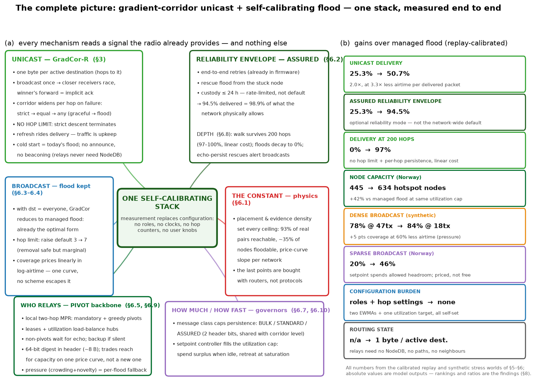
Recommended next steps, in order of information value:
request_id gap (extract it at ingest, optionally
redecode historical rows): this upgrades the response classification of §5.1 from a
98.7%-accurate heuristic to canonical labels. The extraction fix itself (response orientation,
arrival-gated endpoints, route_back ingestion) already shipped to production
during this work.RadioInterface::getTxDelayMsecWeighted, re-keyed on
gradient); the experiment to run is suppression reliability: how often does the losing
candidate fail to hear the winner and forward a duplicate? §6.12 has since bounded what
that measurement can change — the airtime advantage lands somewhere between 3.3× and
1.15× and delivery is insensitive — so the bench test now calibrates a known curve
instead of deciding whether the result stands. It remains the highest-value experiment because
it is the only one that replaces a model with a radio.§6.12 exists because a Meshtastic maintainer read this paper closely enough to find the three places where it was resting on an assumption rather than a measurement, and said so precisely. Two of those three now support the work more firmly than the original argument did; the third corrected a claim that should not have been made in the form it was. §6.13 is an indirect consequence of the same review: having been shown one assumption we had not measured, we went looking for others and found a larger one in our own workload. Review of that quality is scarce and this paper is materially better for it.
This work was produced with substantial AI assistance (Cursor agents). The AI wrote the simulation and experiment code, ran the data extraction and analysis, generated the figures and drafted the text. The author directed the research questions, supplied the production data access, reviewed intermediate results, challenged and corrected the methodology at several points (including the link-extraction fix of §5.1 and the decision to ablate the state clocks) and takes full responsibility for the final content. All numbers are reproducible from the published code and data exports [5] independent of any AI involvement.
sim_norway.py,
experiment_asymmetry.py, experiment_widening.py,
experiment_multinet.py, experiment_cancellation.py,
experiment_plant.py, experiment_target99.py,
experiment_custody.py, experiment_hoplimit_multinet.py,
experiment_broadcast.py, experiment_alltoall.py,
experiment_alltoall_multinet.py, experiment_temporal.py,
experiment_depth.py, experiment_persist.py,
experiment_pressure.py, experiment_pressure_multinet.py,
experiment_headroom.py, experiment_setpoint_multinet.py,
experiment_capacity.py, experiment_capacity_compare.py,
experiment_integrated_stack.py,
experiment_pivot.py, experiment_pivot_multinet.py,
experiment_aggregate.py,
experiment_suppression.py, experiment_mobility.py,
experiment_mobility_sim.py, experiment_matched.py,
fig_*.py; cross-network exports under
data_networks/, position-mobility exports under
data_mobility/) is published at
github.com/relaymonkey/mesh-routing-paper.hop_start. Cited as concurrent work; nothing in this paper is evaluated
against a 2.8 build.